|
Size: 4398
Comment:
|
Size: 2124
Comment:
|
| Deletions are marked like this. | Additions are marked like this. |
| Line 3: | Line 3: |
| Post code that demonstrates the use of the interact command in Sage here. It should be easy for people to just scroll through and paste examples out of here into their own sage notebooks. | '''WARNING: THESE are all broken as of Sept 2016. Fixing this is hopefully a high priority.''' |
| Line 5: | Line 5: |
| We'll likely restructure and reorganize this once we have some nontrivial content and get a sense of how it is laid out. | This is a collection of pages demonstrating the use of [[http://sagemath.org/doc/reference/sagenb/notebook/interact.html#sagenb.notebook.interact.interact|the interact command]] in Sage. It should be easy to just scroll through and copy/paste examples into Sage notebooks. If you have suggestions on how to improve interact, add them [[interactSuggestions|here]] or email [email protected] . Of course, your own examples are also welcome! |
| Line 7: | Line 7: |
| == Graphics == | * [[interact/algebra|Algebra]] * [[interact/bio|Bioinformatics]] * [[interact/calculus|Calculus]] * [[interact/chemistry|Chemistry]] * [[interact/diffeq|Differential Equations]] * [[interact/graphics|Drawing Graphics]] * [[interact/dynsys|Dynamical Systems]] * [[interact/fractal|Fractals]] * [[interact/games|Games and Diversions]] * [[interact/geometry|Geometry]] * [[interact/graph_theory|Graph Theory]] * [[interact/linear_algebra|Linear Algebra]] * [[interact/Loop Quantum Gravity|Loop Quantum Gravity]] * [[interact/misc|Miscellaneous]] * [[interact/number_theory|Number Theory]] * [[interact/stats|Statistics/Probability]] * [[interact/topology|Topology]] * [[interact/web|Web Applications]] |
| Line 9: | Line 26: |
| == Calculus == === A contour map and 3d plot of two inverse distance functions === |
== Explanatory example: Taylor Series == |
| Line 12: | Line 28: |
| {{{ | This is the code and a mockup animation of the interact command. It defines a slider, seen on top, that can be dragged. Once dragged, it changes the value of the variable "order" and the whole block of code gets evaluated. This principle can be seen in various examples presented on the pages above! {{{#!sagecell var('x') x0 = 0 f = sin(x)*e^(-x) p = plot(f,-1,5, thickness=2) dot = point((x0,f(x=x0)),pointsize=80,rgbcolor=(1,0,0)) |
| Line 14: | Line 37: |
| def _(q1=(-1,(-3,3)), q2=(-2,(-3,3)), cmap=['autumn', 'bone', 'cool', 'copper', 'gray', 'hot', 'hsv', 'jet', 'pink', 'prism', 'spring', 'summer', 'winter']): x,y = var('x,y') f = q1/sqrt((x+1)^2 + y^2) + q2/sqrt((x-1)^2+(y+0.5)^2) C = contour_plot(f, (-2,2), (-2,2), plot_points=30, contours=15, cmap=cmap) show(C, figsize=3, aspect_ratio=1) show(plot3d(f, (x,-2,2), (y,-2,2)), figsize=5, viewer='tachyon') |
def _(order=(1..12)): ft = f.taylor(x,x0,order) pt = plot(ft,-1, 5, color='green', thickness=2) html('$f(x)\;=\;%s$'%latex(f)) html('$\hat{f}(x;%s)\;=\;%s+\mathcal{O}(x^{%s})$'%(x0,latex(ft),order+1)) show(dot + p + pt, ymin = -.5, ymax = 1) |
| Line 23: | Line 44: |
| attachment:mountains.png == Number Theory == === Illustrating the prime number thoerem === {{{ @interact def _(N=(100,(2..2000))): html("<font color='red'>$\pi(x)$</font> and <font color='blue'>$x/(\log(x)-1)$</font> for $x < %s$"%N) show(plot(prime_pi, 0, N, rgbcolor='red') + plot(x/(log(x)-1), 5, N, rgbcolor='blue')) }}} attachment:primes.png === Computing the cuspidal subgroup === {{{ html('<h1>Cuspidal Subgroups of Modular Jacobians J0(N)</h1>') @interact def _(N=selector([1..8*13], ncols=8, width=10, default=10)): A = J0(N) print A.cuspidal_subgroup() }}} attachment:cuspgroup.png === A Charpoly and Hecke Operator Graph === {{{ # Note -- in Sage-2.10.3; multiedges are missing in plots; loops are missing in 3d plots @interact def f(N = prime_range(11,400), p = selector(prime_range(2,12),nrows=1), three_d = ("Three Dimensional", False)): S = SupersingularModule(N) T = S.hecke_matrix(p) G = Graph(T, multiedges=True, loops=not three_d) html("<h1>Charpoly and Hecke Graph: Level %s, T_%s</h1>"%(N,p)) show(T.charpoly().factor()) if three_d: show(G.plot3d(), aspect_ratio=[1,1,1]) else: show(G.plot(),figsize=7) }}} attachment:heckegraph.png === Demonstrating the Diffie-Hellman Key Exchange Protocol === {{{ @interact def diffie_hellman(button=selector(["New example"],label='',buttons=True), bits=("Number of bits of prime", (8,12,..512))): maxp = 2^bits p = random_prime(maxp) k = GF(p) g = k.multiplicative_generator() a = ZZ.random_element(10, maxp) b = ZZ.random_element(10, maxp) print """ <html> <style> .gamodp { background:yellow } .gbmodp { background:orange } .dhsame { color:green; font-weight:bold } </style> <h2>%s-Bit Diffie-Hellman Key Exchange</h2> <ol style="color:#000;font:12px Arial, Helvetica, sans-serif"> <li>Alice and Bob agree to use the prime number p=%s and base g=%s.</li> <li>Alice chooses the secret integer a=%s, then sends Bob (<span class="gamodp">g<sup>a</sup> mod p</span>):<br/>%s<sup>%s</sup> mod %s = <span class="gamodp">%s</span>.</li> <li>Bob chooses the secret integer b=%s, then sends Alice (<span class="gbmodp">g<sup>b</sup> mod p</span>):<br/>%s<sup>%s</sup> mod %s = <span class="gbmodp">%s</span>.</li> <li>Alice computes (<span class="gbmodp">g<sup>b</sup> mod p</span>)<sup>a</sup> mod p:<br/>%s<sup>%s</sup> mod %s = <span class="dhsame">%s</span>.</li> <li>Bob computes (<span class="gamodp">g<sup>a</sup> mod p</span>)<sup>b</sup> mod p:<br/>%s<sup>%s</sup> mod %s = <span class="dhsame">%s</span>.</li> </ol></html> """ % (bits, p, g, a, g, a, p, (g^a), b, g, b, p, (g^b), (g^b), a, p, (g^ b)^a, g^a, b, p, (g^a)^b) }}} attachment:dh.jpg === Somewhat Silly Egg Painter === {{{ var('s,t') g(s) = ((0.57496*sqrt(121 - 16.0*s^2))/sqrt(10.+ s)) def P(color, rng): return parametric_plot3d((cos(t)*g(s), sin(t)*g(s), s), (s,rng[0],rng[1]), (t,0,2*pi), plot_points = [150,150], rgbcolor=color, frame = False, opacity = 1) colorlist = ['red','blue','red','blue'] @interact def _(band_number = selector(range(1,5)), current_color = Color('red')): html('<h1 align=center>Egg Painter</h1>') colorlist[band_number-1] = current_color egg = sum([P(colorlist[i],[-2.75+5.5*(i/4),-2.75+5.5*(i+1)/4]) for i in range(4)]) show(egg) }}} attachment:eggpaint.jpg |
{{attachment:taylor_series_animated.gif}} |
Sage Interactions
WARNING: THESE are all broken as of Sept 2016. Fixing this is hopefully a high priority.
This is a collection of pages demonstrating the use of the interact command in Sage. It should be easy to just scroll through and copy/paste examples into Sage notebooks. If you have suggestions on how to improve interact, add them here or email [email protected] . Of course, your own examples are also welcome!
Explanatory example: Taylor Series
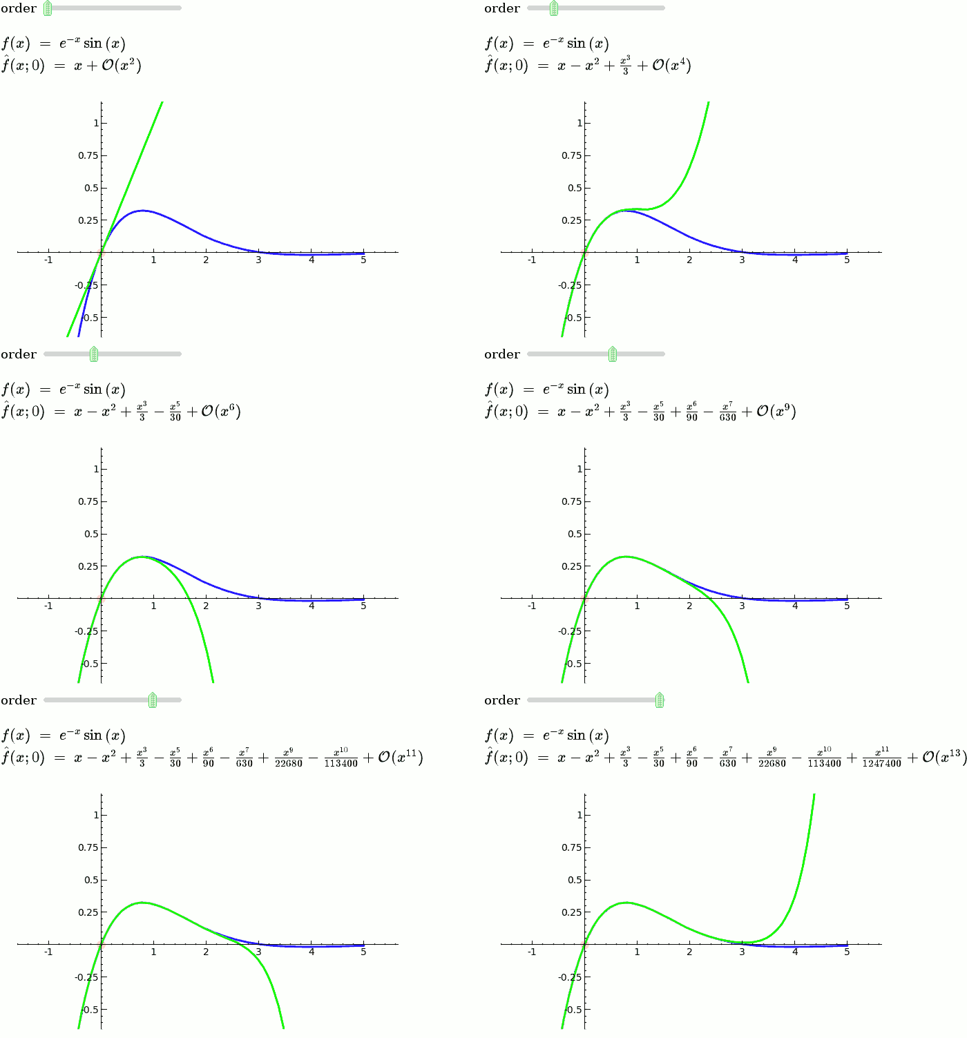
This is the code and a mockup animation of the interact command. It defines a slider, seen on top, that can be dragged. Once dragged, it changes the value of the variable "order" and the whole block of code gets evaluated. This principle can be seen in various examples presented on the pages above!

