|
Size: 1966
Comment:
|
Size: 2532
Comment:
|
| Deletions are marked like this. | Additions are marked like this. |
| Line 3: | Line 3: |
| This is a collection of pages demonstrating the use of [[http://sagemath.org/doc/reference/sagenb/notebook/interact.html#sagenb.notebook.interact.interact|the interact command]] in Sage. It should be easy to just scroll through and copy/paste examples into Sage notebooks. If you have suggestions on how to improve interact, add them [[interactSuggestions|here]] or email [email protected] . Of course, your own examples are also welcome! | This is a collection of pages demonstrating the use of the **interact** command in Sage. It should be easy to just scroll through and copy/paste examples into Sage notebooks. If you have suggestions on how to improve interact, add them [[interact/Suggestions|here]] or email the sage-support mailing list. Of course, your own examples are also welcome! Documentation links: * [[http://doc.sagemath.org/html/en/reference/repl/sage/repl/ipython_kernel/interact.html| interacts in the Jupyter notebook]] (see this page and the two following ones) * [[https://github.com/sagemath/sagenb/blob/master/sagenb/notebook/interact.py|interacts in the legacy SageNB notebook]] (many helpful examples) * [[https://github.com/sagemath/sagecell/blob/master/interact_compatibility.py|Sage Cell Server implementation]] * CoCalc Sage worksheet implementation (needs link) Examples: |
| Line 8: | Line 20: |
| * [[interact/chemistry|Chemistry]] | * [[interact/cryptography|Cryptography]] |
| Line 17: | Line 29: |
| * [[interact/Loop Quantum Gravity|Loop Quantum Gravity]] | |
| Line 28: | Line 41: |
| var('x') | x = SR.var('x') |
| Line 30: | Line 43: |
| f = sin(x)*e^(-x) p = plot(f,-1,5, thickness=2) dot = point((x0,f(x=x0)),pointsize=80,rgbcolor=(1,0,0)) |
f = sin(x) * e^(-x) p = plot(f, -1, 5, thickness=2) dot = point((x0, f(x=x0)), pointsize=80, rgbcolor=(1, 0, 0)) |
| Line 34: | Line 48: |
| def _(order=(1..12)): ft = f.taylor(x,x0,order) pt = plot(ft,-1, 5, color='green', thickness=2) html('$f(x)\;=\;%s$'%latex(f)) html('$\hat{f}(x;%s)\;=\;%s+\mathcal{O}(x^{%s})$'%(x0,latex(ft),order+1)) show(dot + p + pt, ymin = -.5, ymax = 1) |
def _(order=slider([1 .. 12])): ft = f.taylor(x, x0, order) pt = plot(ft, -1, 5, color='green', thickness=2) pretty_print(html(r'$f(x)\;=\;%s$' % latex(f))) pretty_print(html(r'$\hat{f}(x;%s)\;=\;%s+\mathcal{O}(x^{%s})$' % (x0, latex(ft), order+1))) show(dot + p + pt, ymin=-.5, ymax=1) |
Sage Interactions
This is a collection of pages demonstrating the use of the **interact** command in Sage. It should be easy to just scroll through and copy/paste examples into Sage notebooks. If you have suggestions on how to improve interact, add them here or email the sage-support mailing list. Of course, your own examples are also welcome!
Documentation links:
interacts in the Jupyter notebook (see this page and the two following ones)
interacts in the legacy SageNB notebook (many helpful examples)
CoCalc Sage worksheet implementation (needs link)
Examples:
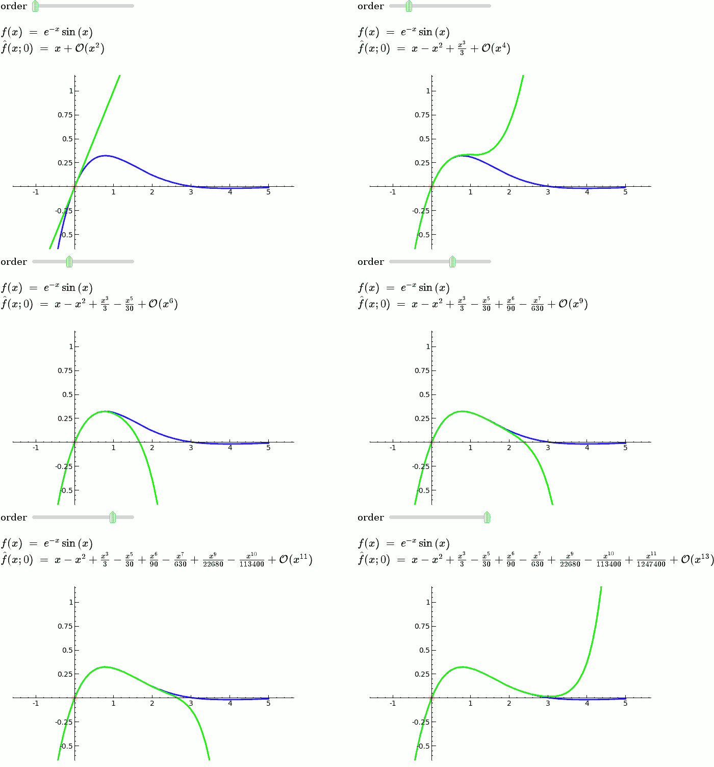
Explanatory example: Taylor Series
This is the code and a mockup animation of the interact command. It defines a slider, seen on top, that can be dragged. Once dragged, it changes the value of the variable "order" and the whole block of code gets evaluated. This principle can be seen in various examples presented on the pages above!

