|
Size: 629
Comment:
|
Size: 1690
Comment:
|
| Deletions are marked like this. | Additions are marked like this. |
| Line 3: | Line 3: |
| Post code that demonstrates the use of the interact command in Sage here. It should be easy for people to just scroll through and paste examples out of here into their own sage notebooks. | This is a collection of pages demonstrating the use of the interact command in Sage. It should be easy to just scroll through and copy/paste examples into sage notebooks. If you have suggestions on how to improve interact, add them [[interactSuggestions|here]] or email [email protected] . Of course, your own examples are also welcome! |
| Line 5: | Line 5: |
| We'll likely restructure and reorganize this once we have some nontrivial content and get a sense of how it is laid out. | * [[interact/graph_theory|Graph Theory]] * [[interact/fractal|Fractals]] * [[interact/calculus|Calculus]] * [[interact/diffeq|Differential Equations]] * [[interact/dynsys|Dynamical Systems]] * [[interact/linear_algebra|Linear Algebra]] * [[interact/algebra|Algebra]] * [[interact/number_theory|Number Theory]] * [[interact/web|Web Applications]] * [[interact/bio|Bioinformatics]] * [[interact/geometry|Geometry]] * [[interact/graphics|Drawing Graphics]] * [[interact/misc|Miscellaneous]] |
| Line 7: | Line 19: |
| == Graphics == | == Explanatory example: Taylor Series == |
| Line 9: | Line 21: |
| == Calculus == == Number Theory == |
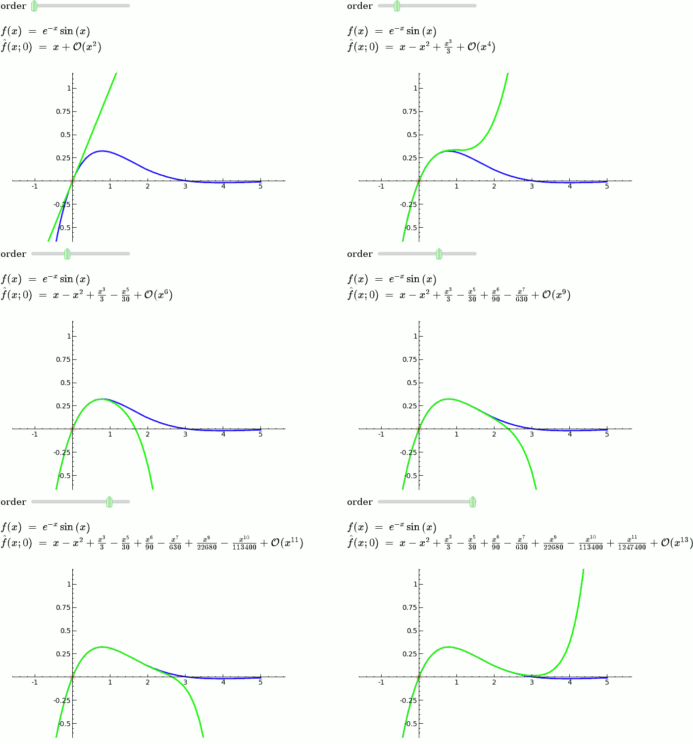
This is the code and a mockup animation of the interact command. It defines a slider, seen on top, that can be dragged. Once dragged, it changes the value of the variable "order" and the whole block of code gets evaluated. This principle can be seen in various examples presented on the pages above! |
| Line 14: | Line 24: |
| html('<h1>Cuspidal Subgroups of Modular Jacobians J0(N)</h1>') | var('x') x0 = 0 f = sin(x)*e^(-x) p = plot(f,-1,5, thickness=2) dot = point((x0,f(x0)),pointsize=80,rgbcolor=(1,0,0)) |
| Line 16: | Line 30: |
| def _(N=selector([1..8*13], ncols=8, width=10, default=10)): A = J0(N) print A.cuspidal_subgroup() |
def _(order=(1..12)): ft = f.taylor(x,x0,order) pt = plot(ft,-1, 5, color='green', thickness=2) html('$f(x)\;=\;%s$'%latex(f)) html('$\hat{f}(x;%s)\;=\;%s+\mathcal{O}(x^{%s})$'%(x0,latex(ft),order+1)) show(dot + p + pt, ymin = -.5, ymax = 1) |
| Line 20: | Line 37: |
attachment:cuspgroup.png |
{{attachment:taylor_series_animated.gif}} |
Sage Interactions
This is a collection of pages demonstrating the use of the interact command in Sage. It should be easy to just scroll through and copy/paste examples into sage notebooks. If you have suggestions on how to improve interact, add them here or email [email protected] . Of course, your own examples are also welcome!
Explanatory example: Taylor Series
This is the code and a mockup animation of the interact command. It defines a slider, seen on top, that can be dragged. Once dragged, it changes the value of the variable "order" and the whole block of code gets evaluated. This principle can be seen in various examples presented on the pages above!
var('x')
x0  = 0
f   = sin(x)*e^(-x)
p   = plot(f,-1,5, thickness=2)
dot = point((x0,f(x0)),pointsize=80,rgbcolor=(1,0,0))
@interact
def _(order=(1..12)):
  ft = f.taylor(x,x0,order)
  pt = plot(ft,-1, 5, color='green', thickness=2)
  html('$f(x)\;=\;%s$'%latex(f))
  html('$\hat{f}(x;%s)\;=\;%s+\mathcal{O}(x^{%s})$'%(x0,latex(ft),order+1))
  show(dot + p + pt, ymin = -.5, ymax = 1)
