|
Size: 2005
Comment:
|
Size: 1977
Comment: rvv (agf)
|
| Deletions are marked like this. | Additions are marked like this. |
| Line 1: | Line 1: |
| #Choose the size D of the square matrix: D = 3 |
= Sage Interactions = |
| Line 4: | Line 3: |
| example = [[1 if k==j else 0 for k in range(D)] for j in range(D)] example[0][-1] = 2 example[-1][0] = 3 |
This is a collection of pages demonstrating the use of [[http://sagemath.org/doc/reference/sagenb/notebook/interact.html#sagenb.notebook.interact.interact|the interact command]] in Sage. It should be easy to just scroll through and copy/paste examples into Sage notebooks. If you have suggestions on how to improve interact, add them [[interactSuggestions|here]] or email [email protected] . Of course, your own examples are also welcome! |
| Line 8: | Line 5: |
| * [[interact/algebra|Algebra]] * [[interact/bio|Bioinformatics]] * [[interact/calculus|Calculus]] * [[interact/chemistry|Chemistry]] * [[interact/diffeq|Differential Equations]] * [[interact/graphics|Drawing Graphics]] * [[interact/dynsys|Dynamical Systems]] * [[interact/fractal|Fractals]] * [[interact/games|Games and Diversions]] * [[interact/geometry|Geometry]] * [[interact/graph_theory|Graph Theory]] * [[interact/linear_algebra|Linear Algebra]] * [[interact/misc|Miscellaneous]] * [[interact/number_theory|Number Theory]] * [[interact/stats|Statistics/Probability]] * [[interact/topology|Topology]] * [[interact/web|Web Applications]] == Explanatory example: Taylor Series == This is the code and a mockup animation of the interact command. It defines a slider, seen on top, that can be dragged. Once dragged, it changes the value of the variable "order" and the whole block of code gets evaluated. This principle can be seen in various examples presented on the pages above! {{{#!python numbers=none var('x') x0 = 0 f = sin(x)*e^(-x) p = plot(f,-1,5, thickness=2) dot = point((x0,f(x=x0)),pointsize=80,rgbcolor=(1,0,0)) |
|
| Line 9: | Line 34: |
| def _(M=input_grid(D,D, default = example, label='Matrix to invert', to_value=matrix), tt = text_control('Enter the bits of precision used' ' (only if you entered floating point numbers)'), precision = slider(5,100,5,20), auto_update=False): if det(M)==0: print 'Failure: Matrix is not invertible' return if M.base_ring() == RR: M = M.apply_map(RealField(precision)) N=M M=M.augment(identity_matrix(D)) print 'We construct the augmented matrix' show(M) for m in range(0,D-1): if M[m,m] == 0: lista = [(M[j,m],j) for j in range(m,D)] maxi, c = max(lista) M[c,:],M[m,:]=M[m,:],M[c,:] print 'We permute rows %d and %d'%(m+1,c+1) show(M) for n in range(m+1,D): a=M[m,m] if M[n,m]!=0: print "We add %s times row %d to row %d"%(-M[n,m]/a, m+1, n+1) M=M.with_added_multiple_of_row(n,m,-M[n,m]/a) show(M) for m in range(D-1,-1,-1): for n in range(m-1,-1,-1): a=M[m,m] if M[n,m]!=0: print "We add %s times row %d to the row %d"%(-M[n,m]/a, m+1, n+1) M=M.with_added_multiple_of_row(n,m,-M[n,m]/a) show(M) for m in range(0,D): if M[m,m]!=1: print 'We divide row %d by %s'%(m+1,M[m,m]) M = M.with_row_set_to_multiple_of_row(m,m,1/M[m,m]) show(M) M=M.submatrix(0,D,D) print 'We keep the right submatrix, which contains the inverse' html('$$M^{-1}=%s$$'%latex(M)) print 'We check it actually is the inverse' html('$$M^{-1}*M=%s*%s=%s$$'%(latex(M),latex(N),latex(M*N))) |
def _(order=(1..12)): ft = f.taylor(x,x0,order) pt = plot(ft,-1, 5, color='green', thickness=2) html('$f(x)\;=\;%s$'%latex(f)) html('$\hat{f}(x;%s)\;=\;%s+\mathcal{O}(x^{%s})$'%(x0,latex(ft),order+1)) show(dot + p + pt, ymin = -.5, ymax = 1) }}} {{attachment:taylor_series_animated.gif}} |
Sage Interactions
This is a collection of pages demonstrating the use of the interact command in Sage. It should be easy to just scroll through and copy/paste examples into Sage notebooks. If you have suggestions on how to improve interact, add them here or email [email protected] . Of course, your own examples are also welcome!
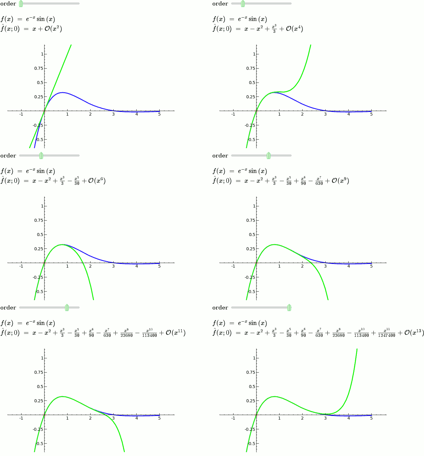
Explanatory example: Taylor Series
This is the code and a mockup animation of the interact command. It defines a slider, seen on top, that can be dragged. Once dragged, it changes the value of the variable "order" and the whole block of code gets evaluated. This principle can be seen in various examples presented on the pages above!
var('x')
x0  = 0
f   = sin(x)*e^(-x)
p   = plot(f,-1,5, thickness=2)
dot = point((x0,f(x=x0)),pointsize=80,rgbcolor=(1,0,0))
@interact
def _(order=(1..12)):
  ft = f.taylor(x,x0,order)
  pt = plot(ft,-1, 5, color='green', thickness=2)
  html('$f(x)\;=\;%s$'%latex(f))
  html('$\hat{f}(x;%s)\;=\;%s+\mathcal{O}(x^{%s})$'%(x0,latex(ft),order+1))
  show(dot + p + pt, ymin = -.5, ymax = 1)

