|
Size: 9827
Comment:
|
← Revision 48 as of 2020-06-05 20:32:41 ⇥
Size: 12926
Comment: negative number in Venn diagram
|
| Deletions are marked like this. | Additions are marked like this. |
| Line 8: | Line 8: |
| by Marshall Hampton. When the two frequencies are well seperated, we hear the right hand side of the identity. When they start getting close, we hear the higher-pitched factor in the left-hand side modulated by the lower-pitched envelope. {{{ |
by Marshall Hampton. When the two frequencies are well separated, we hear the right hand side of the identity. When they start getting close, we hear the higher-pitched factor in the left-hand side modulated by the lower-pitched envelope. {{{#!sagecell |
| Line 17: | Line 17: |
| self.sr = 44100 | self.sr = int(4100) |
| Line 28: | Line 28: |
| def sinsound(freq_ratio = slider(0,1,1/144,1/12)): | def sinsound(freq_ratio = slider(1/144,1,1/144,1/12)): |
| Line 31: | Line 31: |
| html('$\cos(\omega t) - \cos(\omega_0 t) = 2 \sin(\\frac{\omega + \omega_0}{2}t) \sin(\\frac{\omega - \omega_0}{2}t)$') | html(r'$\cos(\omega t) - \cos(\omega_0 t) = 2 \sin(\\frac{\omega + \omega_0}{2}t) \sin(\frac{\omega - \omega_0}{2}t)$') |
| Line 35: | Line 35: |
| s2str = ''.join(wave.struct.pack('h',x) for x in s2f) | s2str = b''.join(wave.struct.pack('f',x) for x in s2f) |
| Line 41: | Line 41: |
| html('<embed src="https:./test'+ lab +'.wav" width="200" height="100"></embed>') html('Frequencies: '+ '$\omega_0 = ' + str(hz1) + ' $, $\omega = '+latex(hz2) + '$') |
pretty_print(html(r'<embed src="cell://test'+ lab +'.wav" width="200" height="100"></embed>')) pretty_print(html(r'Frequencies: $\omega_0 = {} $, $\omega = {}$'.format(str(hz1),latex(hz2)))) |
| Line 49: | Line 49: |
| {{{ | {{{#!sagecell |
| Line 56: | Line 56: |
| self.sr = 44100 | self.sr = int(44100) |
| Line 90: | Line 90: |
| html("Karplus-Strong algorithm with blending and delay stretching") html("<br>K. Karplus and A. Strong, <em>Digital synthesis of plucked string and drum timbres</em>, \nComputer Music Journal 7 (2) (1983), 43–55.<br>") html("Initial waveform:") show(list_plot(s2f[0:2000],plotjoined=True), figsize = [6,4]) html("Waveform after stabilization:") show(list_plot(s2f[20000:22000],plotjoined=True), figsize = [6,4]) s2str = ''.join(wave.struct.pack('h',x) for x in s2f) |
pretty_print(html("Karplus-Strong algorithm with blending and delay stretching")) pretty_print(html("<br>K. Karplus and A. Strong, <em>Digital synthesis of plucked string and drum timbres</em>, \nComputer Music Journal 7 (2) (1983), 43–55.<br>")) pretty_print(html("Initial waveform:")) show(list_plot(s2f[0:2000],plotjoined=True), figsize = [7,3.5]) pretty_print(html("Waveform after stabilization:")) show(list_plot(s2f[20000:22000],plotjoined=True), figsize = [7,3.5]) s2str = b''.join(wave.struct.pack('f',x) for x in s2f) |
| Line 100: | Line 100: |
| html('<embed src="https:./test'+ lab +'.wav" width="200" height="100"></embed>') | pretty_print(html('<embed src="cell://test'+ lab +'.wav" width="200" height="100"></embed>')) |
| Line 107: | Line 107: |
| {{{ | {{{#!sagecell |
| Line 122: | Line 122: |
| html('<center>') html("$X \cap Y$ = %s"%f(XY)) html("$X \cap Z$ = %s"%f(XZ)) html("$Y \cap Z$ = %s"%f(YZ)) html("$X \cap Y \cap Z$ = %s"%f(XYZ)) html('</center>') |
pretty_print(html("<center><p>$X \\cap Y$ = {}</p><p> $X \\cap Z$ = {}</p><p> $Y \\cap Z$ = {}</p><p> $X \\cap Y \\cap Z$ = {}<center>".format(f(XY),f(XZ),f(YZ),f(XYZ)))) |
| Line 163: | Line 158: |
| {{{ | {{{#!sagecell |
| Line 166: | Line 161: |
| print (lambda f:f(0,f))( | print((lambda f:f(0,f))( |
| Line 171: | Line 166: |
| ) | )) |
| Line 177: | Line 172: |
| {{{ html('<h2>Profile the given input</h2>') |
{{{#!sagecell pretty_print(html('<h2>Profile the given input</h2>')) |
| Line 184: | Line 179: |
| print "<html>" # trick to avoid word wrap | |
| Line 186: | Line 180: |
| cProfile.run(cmd) | cProfile.runctx(cmd,globals(), locals()) |
| Line 188: | Line 182: |
| profile.run(cmd) print "</html>" |
profile.runctx(cmd,globals(), locals()) |
| Line 197: | Line 190: |
| {{{ | {{{#!sagecell |
| Line 200: | Line 193: |
| print globals()[system].eval(code) | print(globals()[system].eval(code)) |
| Line 208: | Line 201: |
| {{{ def minkdemo(list1,list2): |
{{{#!sagecell def minkdemo(list1, list2): |
| Line 211: | Line 204: |
| Returns the Minkowski sum of two lists. | Return the Minkowski sum of two lists. |
| Line 216: | Line 209: |
| temp = [stuff1[i] + stuff2[i] for i in range(len(stuff1))] output.append(temp) |
output.append([a + b for a, b in zip(stuff1, stuff2)]) |
| Line 219: | Line 211: |
| @interact def minksumvis(x1tri = slider(-1,1,1/10,0, label = 'Triangle point x coord.'), yb = slider(1,4,1/10,2, label = 'Blue point y coord.')): t_list = [[1,0],[x1tri,1],[0,0]] |
@interact def minksumvis(x1tri=slider(-1,1,1/10,0, label='Triangle point x coord.'), yb=slider(1,4,1/10,2, label='Blue point y coord.')): t_list = [[1,0], [x1tri,1], [0,0]] |
| Line 232: | Line 225: |
| for an_edge in p12poly.vertex_adjacencies(): edge_lines += line([verts[an_edge[0]], verts[an_edge[1][0]]]) edge_lines += line([verts[an_edge[0]], verts[an_edge[1][1]]]) |
for v0, v1 in p12poly.graph().edges(False): edge_lines += line([v0, v1]) |
| Line 254: | Line 246: |
| by Pablo Angulo {{{ %cython |
by Pablo Angulo, Eviatar Bach {{{#!sagecell |
| Line 259: | Line 250: |
def cellular(rule, int N): |
from random import randint def cellular(rule, N, initial='Single-cell'): |
| Line 265: | Line 257: |
| initial: starting condition; can be either single-cell or a random binary row | |
| Line 266: | Line 259: |
| cdef int j,k,l M=zeros( (N,2*N+1), dtype=int) M[0,N]=1 |
M=zeros( (N,2*N+2), dtype=int) if initial=='Single-cell': M[0,N]=1 else: M[0]=[randint(0,1) for a in range(2*N+2)] |
| Line 271: | Line 266: |
| for k in range(N-j,N+j+1): | for k in range(2*N): |
| Line 274: | Line 269: |
| return M }}} {{{ |
return M[:,:-1] |
| Line 284: | Line 278: |
| def _( N=input_box(label='Number of iterations',default=100), | def _( initial=selector(['Single-cell', 'Random'], label='Starting condition'), N=input_box(label='Number of iterations',default=100), |
| Line 286: | Line 280: |
| size = slider(1, 11, step_size=1, default=6 ) ): | size = slider(1, 11, label= 'Size', step_size=1, default=6 ), auto_update=False): |
| Line 288: | Line 282: |
| M = cellular(rule, N) plot_M = matrix_plot(M) |
M = cellular(rule, N, initial) plot_M = matrix_plot(M, cmap='binary') |
| Line 292: | Line 286: |
| {{attachment:cellular.png}} | {{attachment:cellular2.png}} == Another Interactive Venn Diagram == by Jane Long (adapted from http://wiki.sagemath.org/interact/misc) This interact models a problem in which a certain number of people are surveyed to see if they participate in three different activities (running, biking, and swimming). Users can indicate the numbers of people in each category, from 0 to 100. Returns a graphic of a labeled Venn diagram with the number of people in each region. Returns an explanatory error message if user input is inconsistent. {{{#!sagecell @interact def _(T=slider([0..100],default=100,label='People surveyed'),X=slider([0..100],default=28,label='Run'), Y=slider([0..100],default=33,label='Bike'), Z=slider([0..100],default=59,label='Swim'),XY=slider([0..100],default=16,label='Run and Bike'),XZ=slider([0..100],default=13,label='Run and Swim'),YZ=slider([0..100],default=12,label='Bike and Swim'),XYZ=slider([0..100],default=7,label='Run, Bike, and Swim')): centers = [(cos(n*2*pi/3), sin(n*2*pi/3)) for n in [0,1,2]] scale = 1.7 clr = ['yellow', 'blue', 'green'] G = Graphics() for i in range(3): G += circle(centers[i], scale, rgbcolor=clr[i], fill=True, alpha=0.3) for i in range(3): G += circle(centers[i], scale, rgbcolor='black') # Label sets G += text('Run',(3,0),rgbcolor='black') G += text('Bike',(-1,3),rgbcolor='black') G += text('Swim',(-1,-3),rgbcolor='black') # Plot pairs of intersections ZX=XZ-XYZ G += text(ZX, (1.3*cos(2*2*pi/3 + pi/3), 1.3*sin(2*2*pi/3 + pi/3)), rgbcolor='black') YX=XY-XYZ G += text(YX, (1.3*cos(0*2*pi/3 + pi/3), 1.3*sin(0*2*pi/3 + pi/3)), rgbcolor='black') ZY=YZ-XYZ G += text(ZY, (1.3*cos(1*2*pi/3 + pi/3), 1.3*sin(1*2*pi/3 + pi/3)), rgbcolor='black') # Plot what is in one but neither other XX=X-ZX-YX-XYZ G += text(XX, (1.5*centers[0][0],1.7*centers[0][1]), rgbcolor='black') YY=Y-ZY-YX-XYZ G += text(YY, (1.5*centers[1][0],1.7*centers[1][1]), rgbcolor='black') ZZ=Z-ZY-ZX-XYZ G += text(ZZ, (1.5*centers[2][0],1.7*centers[2][1]), rgbcolor='black') # Plot intersection of all three G += text(XYZ, (0,0), rgbcolor='black') # Indicate number not in X, in Y, or in Z C = T-XX-YY-ZZ-ZX-ZY-YX-XYZ G += text(C,(3,-3),rgbcolor='black') # Check reasonableness before displaying result if XYZ>XY or XYZ>XZ or XYZ>YZ or XY>X or XY>Y or XZ>X or XZ>Z or YZ>Y or YZ>Z or C<0 or XYZ<0 or XZ<0 or YZ<0 or XY<0 or X<0 or Y<0 or Z<0 or XX<0 or YY<0 or ZZ<0: print('This situation is impossible! (Why?)') else: G.show(aspect_ratio=1, axes=False) }}} {{attachment:vennjhl.png}} |
Sage Interactions - Miscellaneous
goto interact main page
Contents
Hearing a trigonometric identity
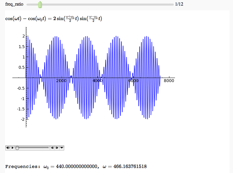
by Marshall Hampton. When the two frequencies are well separated, we hear the right hand side of the identity. When they start getting close, we hear the higher-pitched factor in the left-hand side modulated by the lower-pitched envelope.
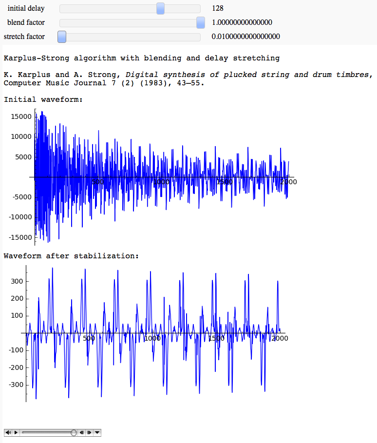
Karplus-Strong algorithm for plucked and percussive sound generation
by Marshall Hampton
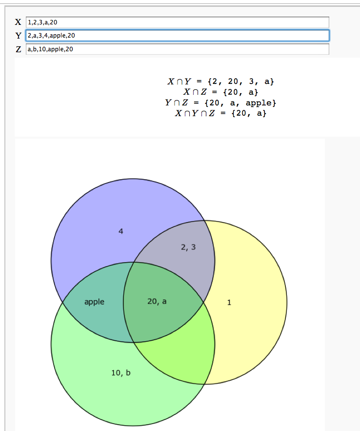
An Interactive Venn Diagram
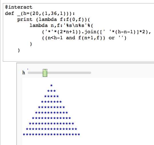
Unreadable code
by Igor Tolkov
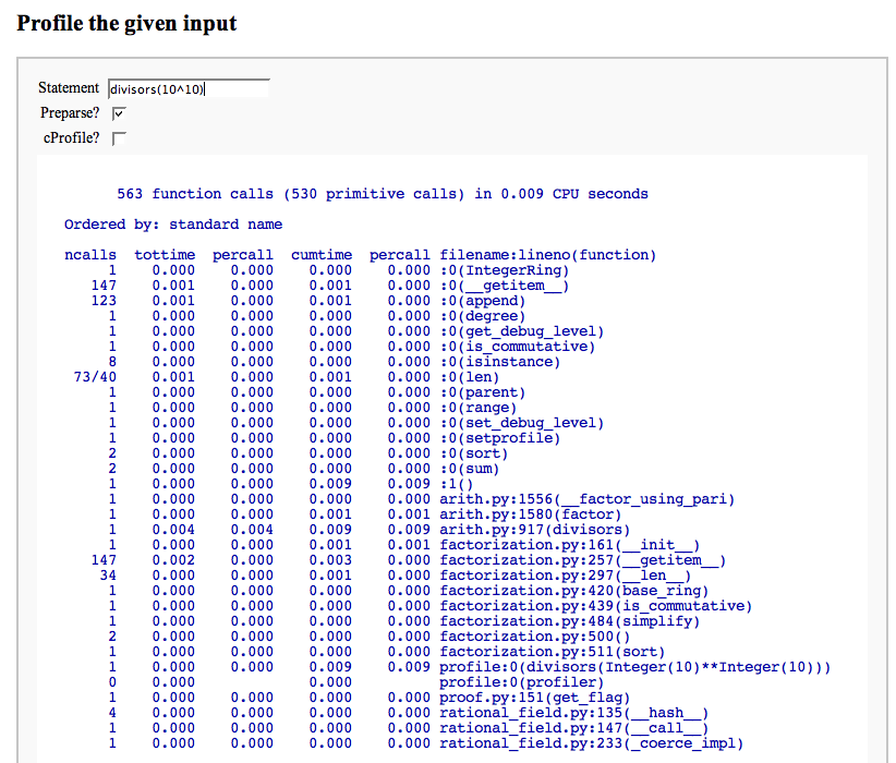
Profile a snippet of code
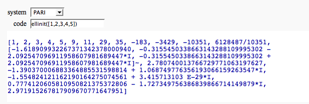
Evaluate a bit of code in a given system
by William Stein (there is no way yet to make the text box big):
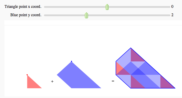
Minkowski Sum
by Marshall Hampton
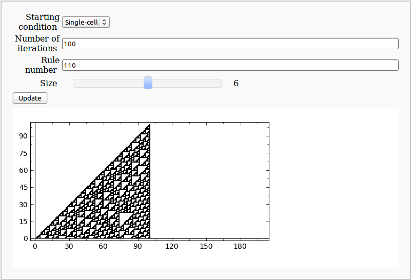
Cellular Automata
by Pablo Angulo, Eviatar Bach
Another Interactive Venn Diagram
by Jane Long (adapted from http://wiki.sagemath.org/interact/misc)
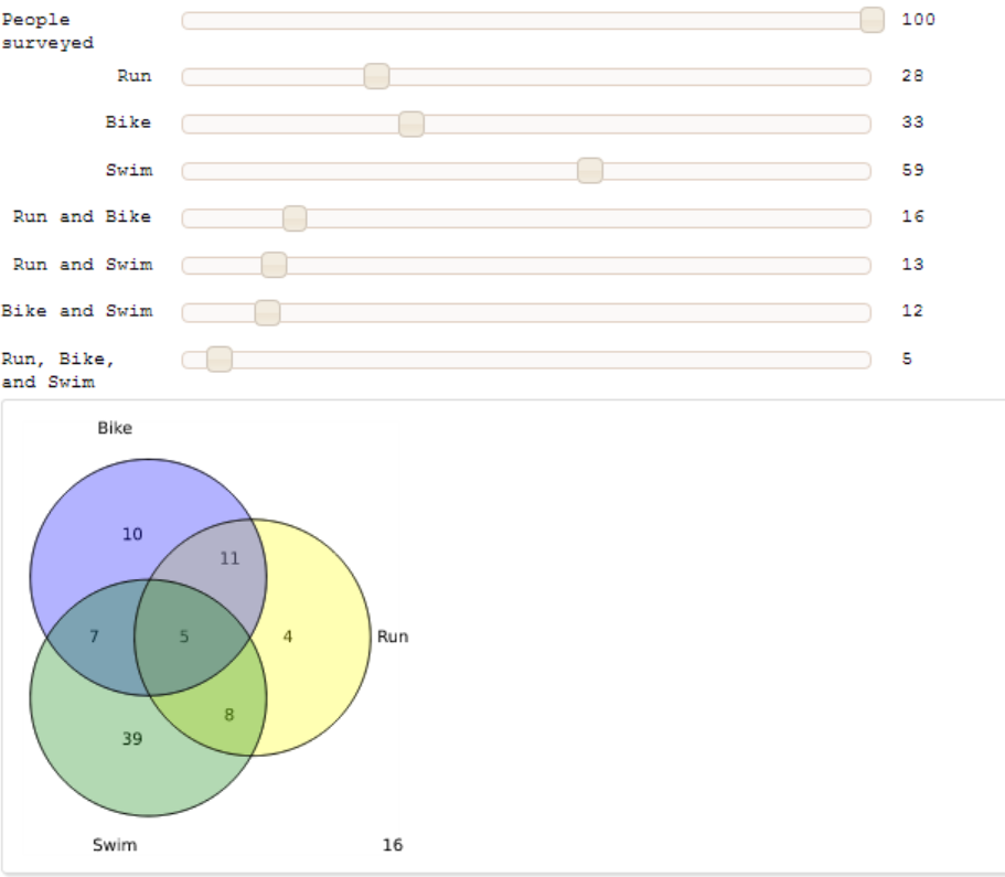
This interact models a problem in which a certain number of people are surveyed to see if they participate in three different activities (running, biking, and swimming). Users can indicate the numbers of people in each category, from 0 to 100. Returns a graphic of a labeled Venn diagram with the number of people in each region. Returns an explanatory error message if user input is inconsistent.
