|
Size: 14961
Comment: ||width=600 for attachment:HSEL
|
Size: 19647
Comment: Solution of a non homogeneous system of linear equations
|
| Deletions are marked like this. | Additions are marked like this. |
| Line 353: | Line 353: |
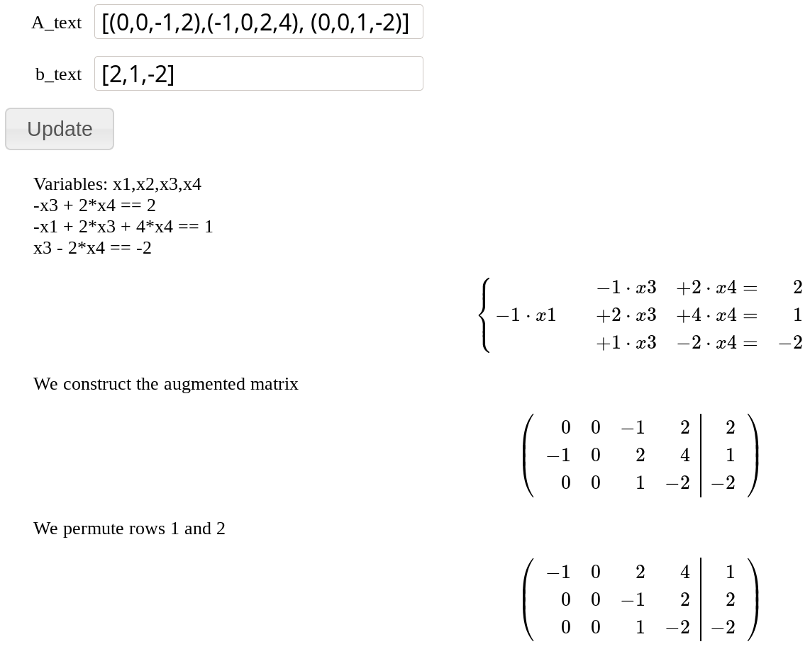
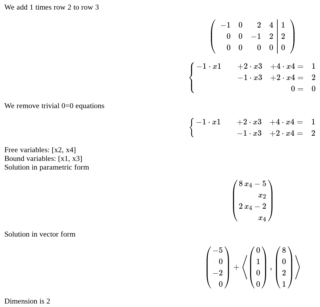
== Solution of a non homogeneous system of linear equations == by Pablo Angulo Coefficients are introduced as a matrix in a single text box, and independent terms as a vector in a separate text box. The number of equations and unknowns are arbitrary. {{{#!sagecell from sage.misc.html import HtmlFragment def SLE_as_latex(A, b, variables): nvars = A.ncols() pretty_print(HtmlFragment( r'$$\left\{\begin{array}{%s}'%('r'*(nvars+1))+ r'\\'.join('%s=&%s'%( (' & '.join((r'%s%s\cdot %s'%('+' if c>0 else '',c,v) if c else '') for c,v in zip(row, variables)) if not row.is_zero() else '&'*(nvars-1)+'0',y) ) for row,y in zip(A,b))+ r'\end{array}\right.$$')) def extended_matrix_as_latex(M): A = M[:,:-1] b = M.column(-1) nvars = A.ncols() pretty_print(HtmlFragment( r'$$\left(\begin{array}{%s}'%('r'*nvars+ '|r')+ r'\\'.join('%s&%s'%( ' & '.join('%s'%c for c in row) ,y) for row,y in zip(A,b))+ r'\end{array}\right)$$')) @interact def SEL(A_text='[(0,0,-1,2),(-1,0,2,4), (0,0,1,-2)]', b_text='[2,1,-2]', auto_update=False ): A = matrix(eval(A_text)) b = vector(eval(b_text)) M = A.augment(b) neqs = len(b) nvars = A.ncols() var_names = ','.join('x%d'%j for j in [1..nvars]) variables = var(var_names) pretty_print(HtmlFragment('Variables: %s'% var_names)) for row,y in zip(A,b): pretty_print(HtmlFragment(sum(c*v for c,v in zip(row, variables))==y)) SLE_as_latex(A, b, variables) pretty_print(HtmlFragment( 'We construct the augmented matrix')) extended_matrix_as_latex(M) pivot = {} ibound_variables = [] for m,row in enumerate(A): for k in range(m,nvars): lista = [(abs(M[j,k]),j) for j in range(m,neqs)] maxi, c = max(lista) if maxi > 0: ibound_variables.append(k) if M[m,k]==0: M[c,:],M[m,:]=M[m,:],M[c,:] pretty_print( HtmlFragment('We permute rows %d and %d'%(m+1,c+1))) extended_matrix_as_latex(M) pivot[m] = k break a=M[m,k] for n in range(m+1,neqs): if M[n,k]!=0: pretty_print( HtmlFragment("We add %s times row %d to row %d"%(-M[n,k]/a, m+1, n+1))) M=M.with_added_multiple_of_row(n,m,-M[n,k]/a) extended_matrix_as_latex(M) A = M[:,:-1] b = M.column(-1) SLE_as_latex(A, b, variables) SEL_type = 'compatible' null_rows = None for k,(row,y) in enumerate(zip(A,b)): if row.is_zero(): if y==0 and null_rows is None: null_rows = k break elif y!=0: SEL_type = 'incompatible' if SEL_type == 'incompatible': pretty_print( HtmlFragment('The system has no solutions')) return if null_rows: pretty_print(HtmlFragment('We remove trivial 0=0 equations')) A = A[:null_rows,:] b = b[:null_rows] SLE_as_latex(A, b, variables) ifree_variables = [k for k in range(nvars) if k not in ibound_variables] bound_variables = [variables[k] for k in ibound_variables] free_variables = [variables[k] for k in ifree_variables] pretty_print( HtmlFragment('Free variables: %s'% free_variables)) pretty_print( HtmlFragment('Bound variables: %s'% bound_variables)) reduced_eqs = [ sum(c*v for c,v in zip(row, variables))==y for row,y in zip(A,b) ] xvector = vector(variables) if len(bound_variables)==1: soldict = solve(reduced_eqs, bound_variables[0], solution_dict=True)[0] else: soldict = solve(reduced_eqs, bound_variables, solution_dict=True)[0] pretty_print( HtmlFragment('Solution in parametric form')) parametric_sol = matrix( xvector.apply_map(lambda s:s.subs(soldict)) ).transpose() show(parametric_sol) pretty_print( HtmlFragment('Solution in vector form')) pretty_print( HtmlFragment( r'$$ %s + \left\langle %s\right\rangle$$'%( latex(parametric_sol.subs(dict(zip(free_variables, [0]*len(free_variables))))), ','.join(latex( parametric_sol.apply_map(lambda s:s.diff(v)) ) for v in free_variables) if free_variables else latex(matrix([0]*nvars).transpose())) )) pretty_print( HtmlFragment('Dimension is %d'%len(free_variables))) }}} {{attachment:NHSEL_1.png||width=600}} {{attachment:NHSEL_2.png||width=600}} |
Sage Interactions - Linear Algebra
goto interact main page
Contents
-
Sage Interactions - Linear Algebra
- Numerical instability of the classical Gram-Schmidt algorithm
- Equality of det(A) and det(A.tranpose())
- Linear transformations
- Gerschgorin Circle Theorem
- Singular value decomposition
- Discrete Fourier Transform
- The Gauss-Jordan method for inverting a matrix
- Solution of an homogeneous system of linear equations
- Solution of a non homogeneous system of linear equations
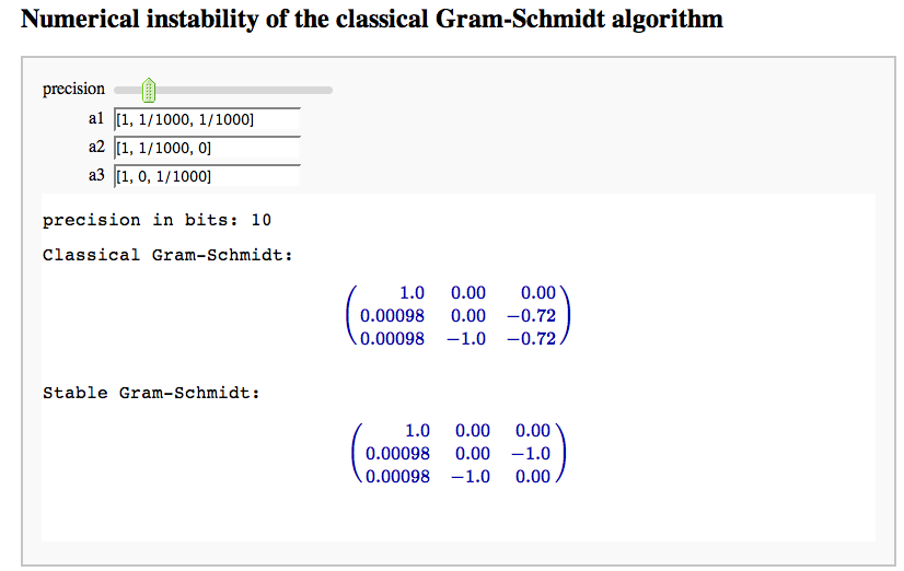
Numerical instability of the classical Gram-Schmidt algorithm
by Marshall Hampton
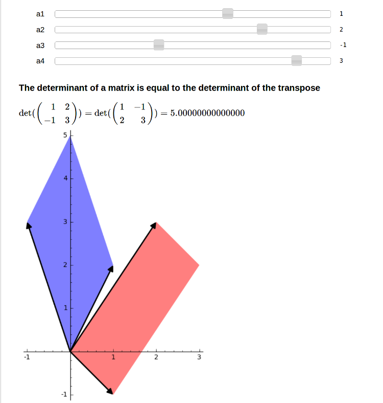
Equality of det(A) and det(A.tranpose())
by Marshall Hampton
Linear transformations
by Jason Grout
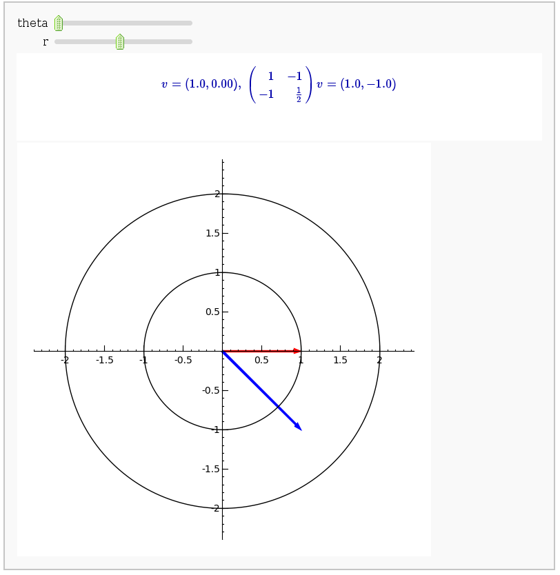
A square matrix defines a linear transformation which rotates and/or scales vectors. In the interact command below, the red vector represents the original vector (v) and the blue vector represents the image w under the linear transformation. You can change the angle and length of v by changing theta and r.
Gerschgorin Circle Theorem
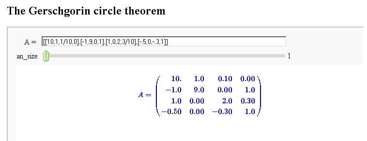
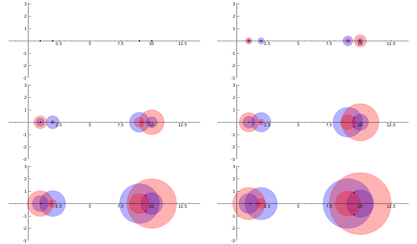
by Marshall Hampton. This animated version requires convert (imagemagick) to be installed, but it can easily be modified to a static version. The animation illustrates the idea behind the stronger version of Gerschgorin's theorem, which says that if the disks around the eigenvalues are disjoint then there is one eigenvalue per disk. The proof is by continuity of the eigenvalues under a homotopy to a diagonal matrix.
Singular value decomposition
by Marshall Hampton
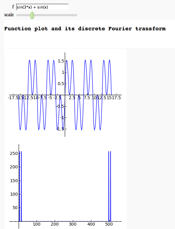
Discrete Fourier Transform
by Marshall Hampton
The Gauss-Jordan method for inverting a matrix
by Hristo Inouzhe
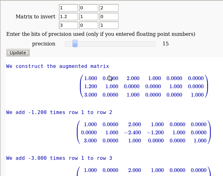
...(goes all the way to invert the matrix)
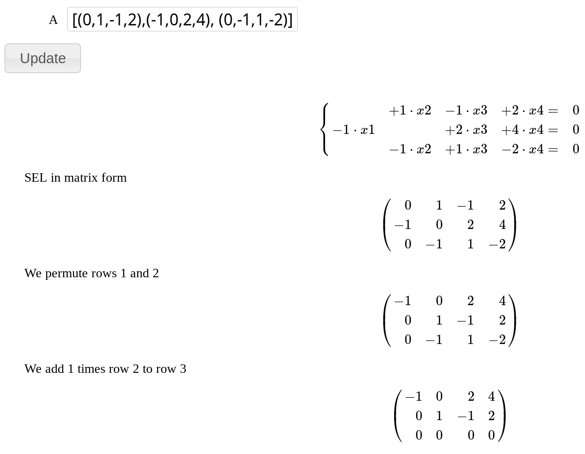
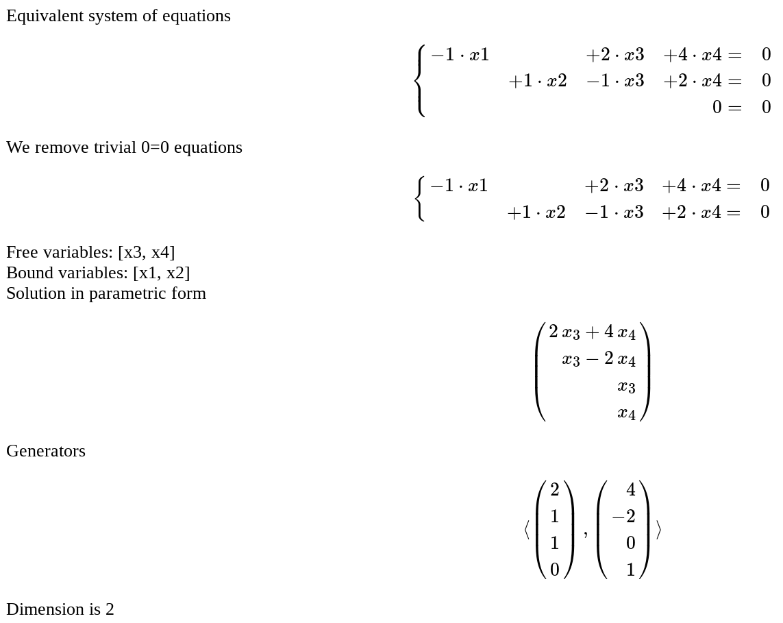
Solution of an homogeneous system of linear equations
by Pablo Angulo
Coefficients are introduced as a matrix in a single text box. The number of equations and unknowns are arbitrary.
Solution of a non homogeneous system of linear equations
by Pablo Angulo
Coefficients are introduced as a matrix in a single text box, and independent terms as a vector in a separate text box. The number of equations and unknowns are arbitrary.
