Differences between revisions 20 and 35 (spanning 15 versions)

Sage Interactions - Linear Algebra

Contents

Sage Interactions - Linear Algebra

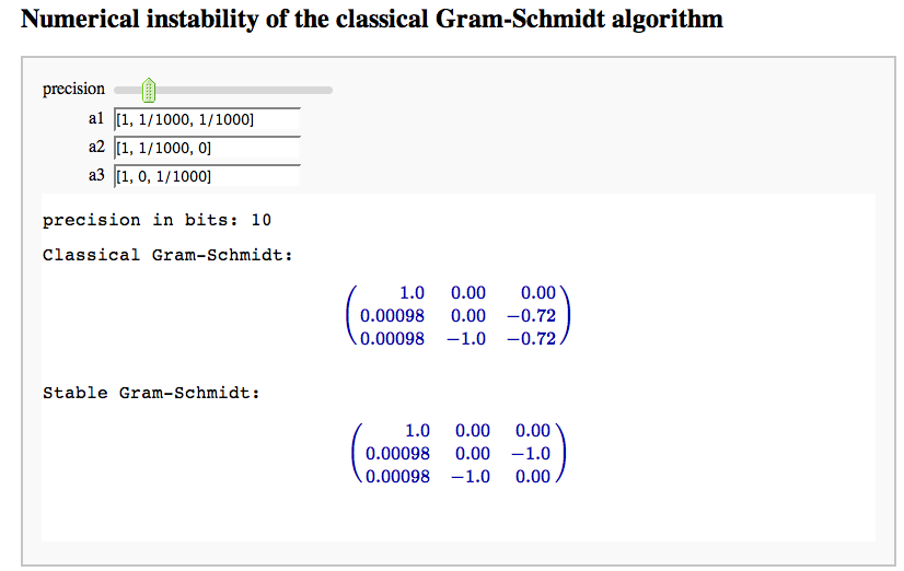
Numerical instability of the classical Gram-Schmidt algorithm

by Marshall Hampton

xxxxxxxxxx
 
def GS_classic(a_list):
    '''
    Given a list of vectors or a matrix, returns the QR factorization using the classical (and numerically unstable) Gram-Schmidt algorithm.    
    '''
    if type(a_list) != list:
        cols = a_list.cols()
        a_list = [x for x in cols]
    indices = range(len(a_list))
    q = []
    r = [[0 for i in indices] for j in indices]
    v = [a_list[i][:] for i in indices]
    for i in indices:
        for j in range(0,i):
            r[j][i] = q[j].inner_product(a_list[i])
            v[i] = v[i] - r[j][i]*q[j]
        r[i][i] = (v[i]*v[i])**(1/2)
        q.append(v[i]/r[i][i])
    q = matrix([q[i] for i in indices]).transpose()
    return q, matrix(r)
def GS_modern(a_list):
    '''
    Given a list of vectors or a matrix, returns the QR factorization using the 'modern' Gram-Schmidt algorithm.    
    '''
    if type(a_list) != list:
        cols = a_list.cols()
        a_list = [x for x in cols]
    indices = range(len(a_list))
    q = []
    r = [[0 for i in indices] for j in indices]
    v = [a_list[i][:] for i in indices]
    for i in indices:
        r[i][i] = v[i].norm(2)
        q.append(v[i]/r[i][i])
        for j in range(i+1, len(indices)):
            r[i][j] = q[i].inner_product(v[j])
            v[j] = v[j] - r[i][j]*q[i]
    q = matrix([q[i] for i in indices]).transpose()
    return q, matrix(r)
pretty_print(html('<h2>Numerical instability of the classical Gram-Schmidt algorithm</h2>'))
@interact
def gstest(precision = slider(range(3,53), default = 10), a1 = input_box([1,1/1000,1/1000]), a2 = input_box([1,1/1000,0]), a3 = input_box([1,0,1/1000])):
    myR = RealField(precision)
    displayR = RealField(5)
    pretty_print(html('precision in bits: ' + str(precision) + '<br>'))
    A = matrix([a1,a2,a3])
    A = [vector(myR,x) for x in A]
    qn, rn = GS_classic(A)
    qb, rb = GS_modern(A)
    pretty_print(html('Classical Gram-Schmidt:'))
    show(matrix(displayR,qn))
    pretty_print(html('Stable Gram-Schmidt:'))
    show(matrix(displayR,qb))

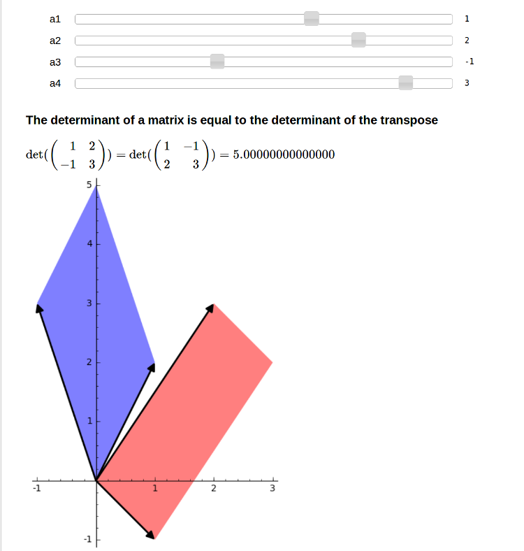
Equality of det(A) and det(A.tranpose())

by Marshall Hampton

xxxxxxxxxx
 
srg = srange(-4,4,1/10,include_endpoint=True)
@interact
def dualv(a1=slider(srg,default=1),a2=slider(srg,default=2), a3=slider(srg,default=-1),a4=slider(srg,default=3)):
    A1 = arrow2d([0,0],[a1,a2],rgbcolor='black')
    A2 = arrow2d([0,0],[a3,a4],rgbcolor='black')
    A3 = arrow2d([0,0],[a1,a3],rgbcolor='black')
    A4 = arrow2d([0,0],[a2,a4],rgbcolor='black')
    p1 = polygon([[0,0],[a1,a2],[a1+a3,a2+a4],[a3,a4],[0,0]], alpha=.5)
    p2 = polygon([[0,0],[a1,a3],[a1+a2,a3+a4],[a2,a4],[0,0]],rgbcolor='red', alpha=.5)
    A = matrix([[a1,a2],[a3,a4]])
    pretty_print(html('<h3>The determinant of a matrix is equal to the determinant of the transpose</h3>'))
    pretty_print(html("$\det(%s) = \det(%s)=%s$"%(latex(A),latex(A.transpose()),latex(RR(A.determinant())))))
    show(A1+A2+A3+A4+p1+p2)

Linear transformations

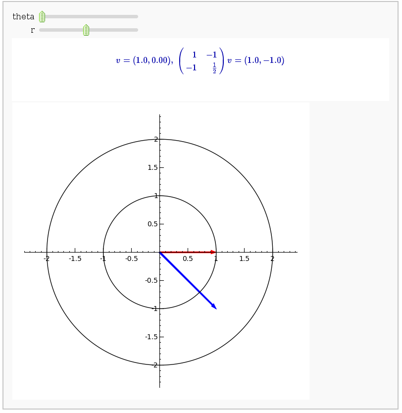
by Jason Grout

A square matrix defines a linear transformation which rotates and/or scales vectors. In the interact command below, the red vector represents the original vector (v) and the blue vector represents the image w under the linear transformation. You can change the angle and length of v by changing theta and r.

xxxxxxxxxx
 
@interact
def linear_transformation(A=matrix([[1,-1],[-1,1/2]]),theta=slider(0, 2*pi, .1), r=slider(0.1, 2, .1, default=1)):
    v=vector([r*cos(theta), r*sin(theta)])
    w = A*v
    circles = sum([circle((0,0), radius=i, color='black') for i in [1..2]])
    pretty_print(html("$%s %s=%s$"%tuple(map(latex, [A, v.column().n(4), w.column().n(4)]))))
    show(v.plot(color='red')+w.plot(color='blue')+circles,aspect_ratio=1)

Gerschgorin Circle Theorem

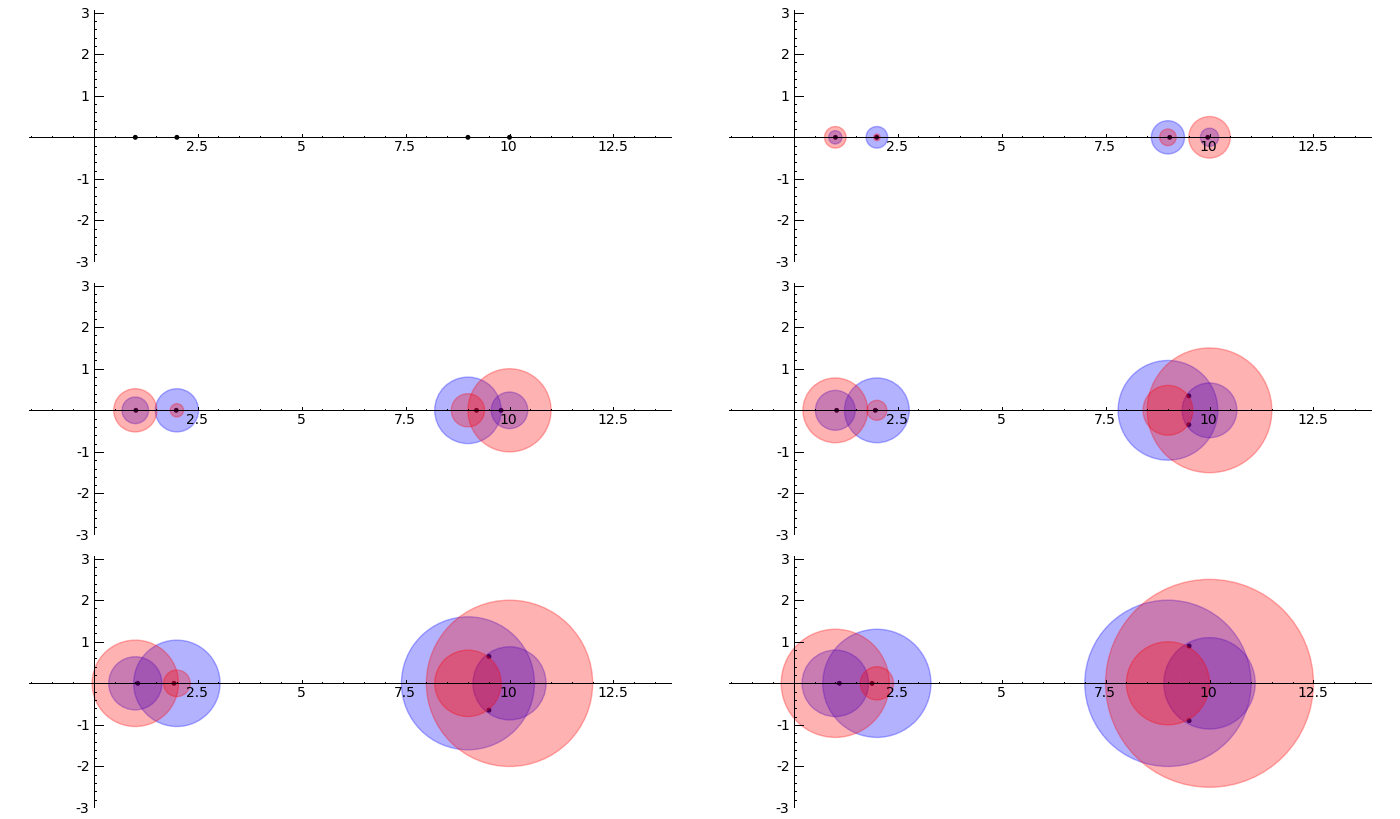
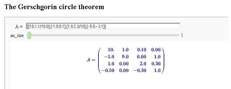
by Marshall Hampton. This animated version requires convert (imagemagick) to be installed, but it can easily be modified to a static version. The animation illustrates the idea behind the stronger version of Gerschgorin's theorem, which says that if the disks around the eigenvalues are disjoint then there is one eigenvalue per disk. The proof is by continuity of the eigenvalues under a homotopy to a diagonal matrix.

xxxxxxxxxx
 
from scipy import linalg
pretty_print(html('<h2>The Gerschgorin circle theorem</h2>'))
@interact
def Gerschgorin(Ain = input_box(default='[[10,1,1/10,0],[-1,9,0,1],[1,0,2,3/10],[-.5,0,-.3,1]]', type = str, label = 'A = '), an_size = slider(1,100,1,1.0)):
    A = sage_eval(Ain)
    size = len(A)
    pretty_print(html('$A = ' + latex(matrix(RealField(10),A))+'$'))
    A = matrix(RealField(10),A)
    B = [[0 for i in range(size)] for j in range(size)]
    for i in range(size):
        B[i][i] = A[i][i]
    B = matrix(B)
    frames = []
​
    centers = [(real(q),imag(q)) for q in [A[i][i] for i in range(size)]]
    radii_row = [sum([abs(A[i][j]) for j in range(i)+range(i+1,size)]) for i in range(size)]
    radii_col = [sum([abs(A[j][i]) for j in range(i)+range(i+1,size)]) for i in range(size)]
    x_min = min([centers[i][0]-radii_row[i] for i in range(size)]+[centers[i][0]-radii_col[i] for i in range(size)])
    x_max = max([centers[i][0]+radii_row[i] for i in range(size)]+[centers[i][0]+radii_col[i] for i in range(size)])
    y_min = min([centers[i][1]-radii_row[i] for i in range(size)]+[centers[i][1]-radii_col[i] for i in range(size)])
    y_max = max([centers[i][1]+radii_row[i] for i in range(size)]+[centers[i][1]+radii_col[i] for i in range(size)])
​
    if an_size > 1: 
        t_range= srange(0,1+1/an_size,1/an_size)
    else:
        t_range = [1]
    for t in t_range:
        C = t*A + (1-t)*B
        eigs = [CDF(x) for x in linalg.eigvals(C.numpy())]
        eigpoints = points([(real(q),imag(q)) for q in eigs],pointsize = 10, rgbcolor = (0,0,0))
        centers = [(real(q),imag(q)) for q in [A[i][i] for i in range(size)]]
        radii_row = [sum([abs(C[i][j]) for j in range(i)+range(i+1,size)]) for i in range(size)]
        radii_col = [sum([abs(C[j][i]) for j in range(i)+range(i+1,size)]) for i in range(size)]
        scale = max([(x_max-x_min),(y_max-y_min)])
        scale = 7/scale
        row_circles = sum([circle(centers[i],radii_row[i],fill=True, alpha = .3) for i in range(size)])
        col_circles = sum([circle(centers[i],radii_col[i],fill=True, rgbcolor = (1,0,0), alpha = .3) for i in range(size)])
        ft = eigpoints+row_circles+col_circles
        frames.append(ft)
    show(animate(frames,figsize = [(x_max-x_min)*scale,(y_max-y_min)*scale], xmin = x_min, xmax=x_max, ymin = y_min, ymax = y_max))

Singular value decomposition

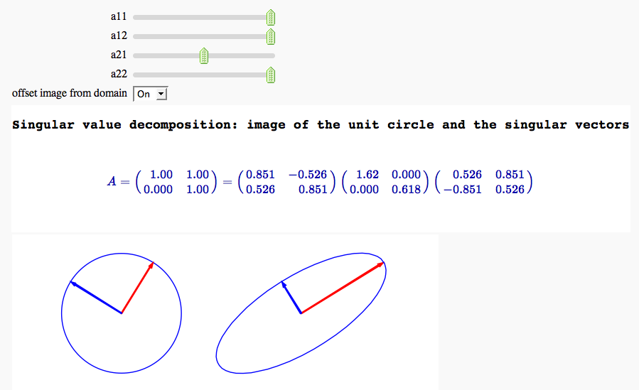
by Marshall Hampton

xxxxxxxxxx
 
import scipy.linalg as lin
var('t')
def rotell(sig,umat,t,offset=0):
    temp = matrix(umat)*matrix(2,1,[sig[0]*cos(t),sig[1]*sin(t)])
    return [offset+temp[0][0],temp[1][0]]
@interact
def svd_vis(a11=slider(-1,1,.05,1),a12=slider(-1,1,.05,1),a21=slider(-1,1,.05,0),a22=slider(-1,1,.05,1),ofs= ('offset image from domain',False)):
    rf_low = RealField(12)
    my_mat = matrix(rf_low,2,2,[a11,a12,a21,a22])
    u,s,vh = lin.svd(my_mat.numpy())
    if ofs: 
        offset = 3
        fsize = 6
        colors = [(1,0,0),(0,0,1),(1,0,0),(0,0,1)]
    else: 
        offset = 0
        fsize = 5
        colors = [(1,0,0),(0,0,1),(.7,.2,0),(0,.3,.7)]
    vvects = sum([arrow([0,0],matrix(vh).row(i),rgbcolor = colors[i]) for i in (0,1)])    
    uvects = Graphics()
    for i in (0,1):
        if s[i] != 0: uvects += arrow([offset,0],vector([offset,0])+matrix(s*u).column(i),rgbcolor = colors[i+2])
    pretty_print(html('<h3>Singular value decomposition: image of the unit circle and the singular vectors</h3>'))
    pretty_print(html("$A = %s  = %s %s %s$"%(latex(my_mat), latex(matrix(rf_low,u.tolist())), latex(matrix(rf_low,2,2,[s[0],0,0,s[1]])), latex(matrix(rf_low,vh.tolist())))))
    image_ell = parametric_plot(rotell(s,u,t, offset),(0,2*pi))
    graph_stuff=circle((0,0),1)+image_ell+vvects+uvects
    graph_stuff.set_aspect_ratio(1)
    show(graph_stuff,frame = False,axes=False,figsize=[fsize,fsize])

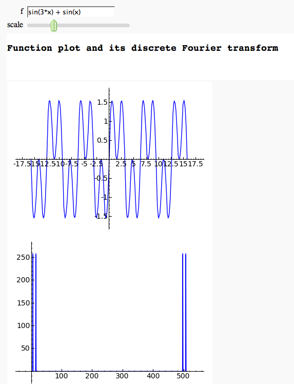
Discrete Fourier Transform

by Marshall Hampton

xxxxxxxxxx
 
import scipy.fftpack as Fourier
@interact
def discrete_fourier(f = input_box(default=sum([sin(k*x) for k in range(1,5,2)])), scale = slider(.1,20,.1,5)):
    pbegin = -float(pi)*scale
    pend = float(pi)*scale
    pretty_print(html("<h3>Function plot and its discrete Fourier transform</h3>"))
    show(plot(f, (x,pbegin, pend), plot_points = 512), figsize = [4,3])
    f_vals = [f(x=ind) for ind in srange(pbegin, pend,(pend-pbegin)/512.0)]
    my_fft = Fourier.fft(f_vals)
    show(list_plot([abs(i) for i in my_fft], plotjoined=True), figsize = [4,3])

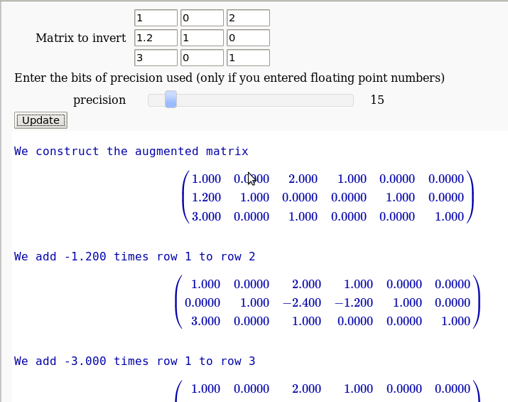
The Gauss-Jordan method for inverting a matrix

by Hristo Inouzhe

xxxxxxxxxx
 
#Choose the size D of the square matrix:
D = 3
​
example = [[1 if k==j else 0 for k in range(D)] for j in range(D)]
example[0][-1] = 2
example[-1][0] = 3
​
@interact
def _(M=input_grid(D,D, default = example,
                   label='Matrix to invert', to_value=matrix),
      tt = text_control('Enter the bits of precision used'
                        ' (only if you entered floating point numbers)'),  
      precision = slider(5,100,5,20),
      auto_update=False):
    if det(M)==0:
        print 'Failure: Matrix is not invertible'
        return
    if M.base_ring() == RR:
        M = M.apply_map(RealField(precision))
    N=M
    M=M.augment(identity_matrix(D))
    print 'We construct the augmented matrix'
    show(M)
    for m in range(0,D-1):
        if M[m,m] == 0:
            lista = [(abs(M[j,m]),j) for j in range(m+1,D)]
            maxi, c = max(lista)
            M[c,:],M[m,:]=M[m,:],M[c,:]
            print 'We permute rows %d and %d'%(m+1,c+1)
            show(M)
        for n in range(m+1,D):
            a=M[m,m]
            if M[n,m]!=0:
                print "We add %s times row %d to row %d"%(-M[n,m]/a, m+1, n+1)
                M=M.with_added_multiple_of_row(n,m,-M[n,m]/a)
                show(M)
    for m in range(D-1,-1,-1):
        for n in range(m-1,-1,-1):
            a=M[m,m]
            if M[n,m]!=0:
                print "We add %s times row %d to the row %d"%(-M[n,m]/a, m+1, n+1)
                M=M.with_added_multiple_of_row(n,m,-M[n,m]/a)
                show(M)       
    for m in range(0,D):
        if M[m,m]!=1:
            print 'We divide row %d by %s'%(m+1,M[m,m])
            M = M.with_row_set_to_multiple_of_row(m,m,1/M[m,m])
            show(M)   
    M=M.submatrix(0,D,D)
    print 'We keep the right submatrix, which contains the inverse'        
    html('$$M^{-1}=%s$$'%latex(M))
    print 'We check it actually is the inverse'
    html('$$M^{-1}*M=%s*%s=%s$$'%(latex(M),latex(N),latex(M*N)))

...(goes all the way to invert the matrix)

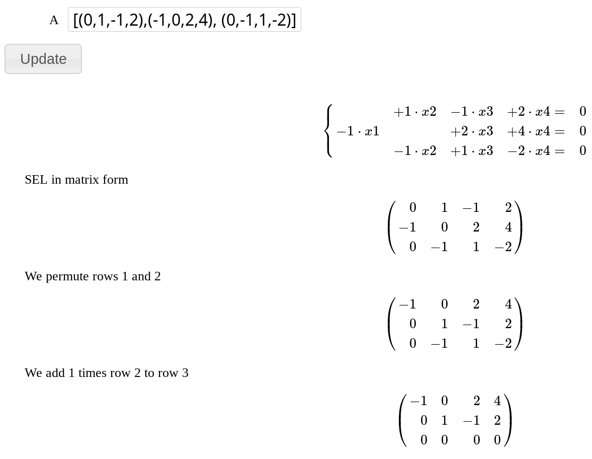
Solution of an homogeneous system of linear equations

by Pablo Angulo and Hristo Inouzhe

Coefficients are introduced as a matrix in a single text box. The number of equations and unknowns are arbitrary.

xxxxxxxxxx
 
from sage.misc.html import HtmlFragment
​
def HSLE_as_latex(A, variables):
    nvars = A.ncols()
    pretty_print(HtmlFragment( 
    r'$$\left\{\begin{array}{%s}'%('r'*(nvars+1))+
    r'\\'.join('%s=&0'%( 
        ' & '.join((r'%s%s\cdot %s'%('+' if c>0 else '',c,v) if c else '') for c,v in zip(row, variables))
        if not row.is_zero() else '&'*(nvars-1)+'0' 
               ) for row in A)+
    r'\end{array}\right.$$'))
​
@interact
def SEL(A='[(0,1,-1,2),(-1,0,2,4), (0,-1,1,-2)]',
        auto_update=False
    ):
    M = A = matrix(eval(A))
    neqs = M.nrows()
    nvars = M.ncols()
    var_names = ','.join('x%d'%j for j in [1..nvars])
    variables = var(var_names)
​
    HSLE_as_latex(M, variables)
    pretty_print(HtmlFragment( 'SEL in matrix form'))
    show(M)
​
    pivot = {}
    ibound_variables = []
    for m,row in enumerate(M):
        for k in range(m,nvars):
            lista = [(abs(M[j,k]),j) for j in range(m,neqs)]
            maxi, c = max(lista)
            if maxi > 0:
                ibound_variables.append(k)
                if M[m,k]==0:
                    M[c,:],M[m,:]=M[m,:],M[c,:]
                    pretty_print( HtmlFragment('We permute rows %d and %d'%(m+1,c+1)))
                    show(M)
                pivot[m] = k
                break
​
        a=M[m,k]
        for n in range(m+1,neqs):
            if M[n,k]!=0:
                pretty_print( HtmlFragment("We add %s times row %d to row %d"%(-M[n,k]/a, m+1, n+1)))
                M=M.with_added_multiple_of_row(n,m,-M[n,k]/a)
                show(M)
​
    pretty_print( HtmlFragment('Equivalent system of equations'))
    HSLE_as_latex(M, variables)
    SEL_type = 'compatible'
    null_rows = None
    for k,row in enumerate(M):
        if row.is_zero():
            pretty_print( HtmlFragment('We remove trivial 0=0 equations'))
            M = M[:k,:]
            HSLE_as_latex(M, variables)
                
    ifree_variables = [k for k in range(nvars) if k not in ibound_variables]
    bound_variables = [variables[k] for k in ibound_variables]
    free_variables = [variables[k] for k in ifree_variables]
    pretty_print( HtmlFragment('Free variables: %s'% free_variables))
    pretty_print( HtmlFragment('Bound variables: %s'% bound_variables))
    reduced_eqs = [
        sum(c*v for c,v in zip(row, variables))==0
        for row in M
    ]
    xvector = vector(variables)
    if len(bound_variables)==1:
        soldict = solve(reduced_eqs, bound_variables[0], solution_dict=True)[0]
    else:
        soldict = solve(reduced_eqs, bound_variables, solution_dict=True)[0]
​
    pretty_print( HtmlFragment('Solution in parametric form'))
    parametric_sol = matrix(
        xvector.apply_map(lambda s:s.subs(soldict))
    ).transpose()
    show(parametric_sol)
    pretty_print( HtmlFragment('Generators'))
    pretty_print( HtmlFragment(
        r'$$\langle %s\rangle$$'%','.join(latex(
            parametric_sol.subs(dict((variables[k],1 if j==k else 0) for k in ifree_variables))
        ) for j in ifree_variables)
    ))
    pretty_print( HtmlFragment('Dimension is %d'%len(free_variables)))

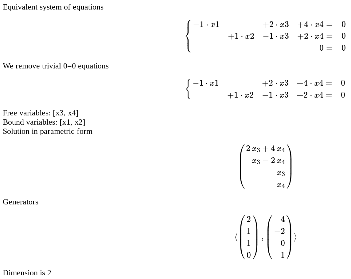
Solution of a non homogeneous system of linear equations

by Pablo Angulo and Hristo Inouzhe

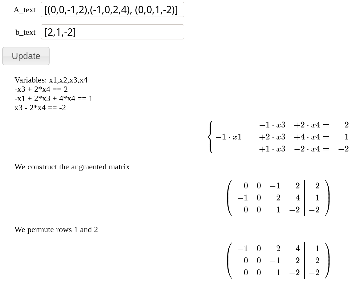
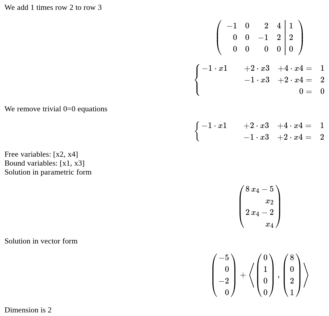
Coefficients are introduced as a matrix in a single text box, and independent terms as a vector in a separate text box. The number of equations and unknowns are arbitrary.

xxxxxxxxxx
 
from sage.misc.html import HtmlFragment
​
def SLE_as_latex(A, b, variables):
    nvars = A.ncols()
    pretty_print(HtmlFragment( 
    r'$$\left\{\begin{array}{%s}'%('r'*(nvars+1))+
    r'\\'.join('%s=&%s'%( 
        (' & '.join((r'%s%s\cdot %s'%('+' if c>0 else '',c,v) if c else '') for c,v in zip(row, variables))
        if not row.is_zero() else '&'*(nvars-1)+'0',y) 
               ) for row,y in zip(A,b))+
    r'\end{array}\right.$$'))
​
def extended_matrix_as_latex(M):
    A = M[:,:-1]
    b = M.column(-1)
    nvars = A.ncols()
    pretty_print(HtmlFragment(
    r'$$\left(\begin{array}{%s}'%('r'*nvars+ '|r')+
    r'\\'.join('%s&%s'%( 
        ' & '.join('%s'%c for c in row)
        ,y) for row,y in zip(A,b))+
    r'\end{array}\right)$$'))
​
@interact
def SEL(A_text='[(0,0,-1,2),(-1,0,2,4), (0,0,1,-2)]',
        b_text='[2,1,-2]',
        auto_update=False
    ):
    A = matrix(eval(A_text))
    b = vector(eval(b_text))
    M = A.augment(b)
    neqs = len(b)
    nvars = A.ncols()
    var_names = ','.join('x%d'%j for j in [1..nvars])
    variables = var(var_names)
    pretty_print(HtmlFragment('Variables: %s'% var_names))
    for row,y in zip(A,b):
        pretty_print(HtmlFragment(sum(c*v for c,v in zip(row, variables))==y))
​
    SLE_as_latex(A, b, variables)
    pretty_print(HtmlFragment( 'We construct the augmented matrix'))
    extended_matrix_as_latex(M)
​
    pivot = {}
    ibound_variables = []
    for m,row in enumerate(A):
        for k in range(m,nvars):
            lista = [(abs(M[j,k]),j) for j in range(m,neqs)]
            maxi, c = max(lista)
            if maxi > 0:
                ibound_variables.append(k)
                if M[m,k]==0:
                    M[c,:],M[m,:]=M[m,:],M[c,:]
                    pretty_print( HtmlFragment('We permute rows %d and %d'%(m+1,c+1)))
                    extended_matrix_as_latex(M)
                pivot[m] = k
                break
​
        a=M[m,k]
        for n in range(m+1,neqs):
            if M[n,k]!=0:
                pretty_print( HtmlFragment("We add %s times row %d to row %d"%(-M[n,k]/a, m+1, n+1)))
                M=M.with_added_multiple_of_row(n,m,-M[n,k]/a)
                extended_matrix_as_latex(M)
​
    A = M[:,:-1]
    b = M.column(-1)
    SLE_as_latex(A, b, variables)
    SEL_type = 'compatible'
    null_rows = None
    for k,(row,y) in enumerate(zip(A,b)):
        if row.is_zero():
            if y==0 and null_rows is None:
                null_rows = k
                break
            elif y!=0:
                SEL_type = 'incompatible'
    if SEL_type == 'incompatible':
        pretty_print( HtmlFragment('The system has no solutions'))
        return
    if null_rows:
        pretty_print(HtmlFragment('We remove trivial 0=0 equations'))
        A = A[:null_rows,:]
        b = b[:null_rows]
        SLE_as_latex(A, b, variables)
​
    ifree_variables = [k for k in range(nvars) if k not in ibound_variables]
    bound_variables = [variables[k] for k in ibound_variables]
    free_variables = [variables[k] for k in ifree_variables]
    pretty_print( HtmlFragment('Free variables: %s'% free_variables))
    pretty_print( HtmlFragment('Bound variables: %s'% bound_variables))
    reduced_eqs = [
        sum(c*v for c,v in zip(row, variables))==y
        for row,y in zip(A,b)
    ]
    xvector = vector(variables)
    if len(bound_variables)==1:
        soldict = solve(reduced_eqs, bound_variables[0], solution_dict=True)[0]
    else:
        soldict = solve(reduced_eqs, bound_variables, solution_dict=True)[0]
    pretty_print( HtmlFragment('Solution in parametric form'))
    parametric_sol = matrix(
        xvector.apply_map(lambda s:s.subs(soldict))
    ).transpose()
    show(parametric_sol)
    pretty_print( HtmlFragment('Solution in vector form'))
    pretty_print( HtmlFragment(
        r'$$ %s + \left\langle %s\right\rangle$$'%(
            latex(parametric_sol.subs(dict(zip(free_variables, [0]*len(free_variables))))),
            ','.join(latex(
            parametric_sol.apply_map(lambda s:s.diff(v))
        ) for v in free_variables) if free_variables else latex(matrix([0]*nvars).transpose()))
    ))
    pretty_print( HtmlFragment('Dimension is %d'%len(free_variables)))

-  ⇤ ← Revision 20 as of 2012-05-09 03:47:40 → 
  Size: 10445
  Editor: jason
  Comment:
+   ← Revision 35 as of 2020-11-27 12:10:23 → ⇥
  Size: 19683
  Editor: pang
  Comment: credit to Hristo Inouzhe by Pablo Angulo on the last two interacts
-Deletions are marked like this.
+Additions are marked like this.
 Line 6:
-== Numerical instability of the classical Gram-Schmidt algorithm FIXME ==
by Marshall Hampton (tested by William Stein, who thinks this is really nice!)
+== Numerical instability of the classical Gram-Schmidt algorithm ==
by Marshall Hampton
 Line 19:
-    v = [a_list[i].copy() for i in indices]
+    v = [a_list[i][:] for i in indices]
 Line 24:
-        r[i][i] = (v[i]*v[i])^(1/2)
+        r[i][i] = (v[i]*v[i])**(1/2)
 Line 38:
-    v = [a_list[i].copy() for i in indices]
+    v = [a_list[i][:] for i in indices]
 Line 47:
-html('<h2>Numerical instability of the classical Gram-Schmidt algorithm</h2>')
+pretty_print(html('<h2>Numerical instability of the classical Gram-Schmidt algorithm</h2>'))
 Line 52:
-    html('precision in bits: ' + str(precision) + '<br>')
+    pretty_print(html('precision in bits: ' + str(precision) + '<br>'))
 Line 57:
-    html('Classical Gram-Schmidt:')
+    pretty_print(html('Classical Gram-Schmidt:'))
 Line 59:
-    html('Stable Gram-Schmidt:')
+    pretty_print(html('Stable Gram-Schmidt:'))
 Line 63:
+== Equality of det(A) and det(A.tranpose()) ==
by Marshall Hampton
{{{#!sagecell
srg = srange(-4,4,1/10,include_endpoint=True)
@interact
def dualv(a1=slider(srg,default=1),a2=slider(srg,default=2), a3=slider(srg,default=-1),a4=slider(srg,default=3)):
    A1 = arrow2d([0,0],[a1,a2],rgbcolor='black')
    A2 = arrow2d([0,0],[a3,a4],rgbcolor='black')
    A3 = arrow2d([0,0],[a1,a3],rgbcolor='black')
    A4 = arrow2d([0,0],[a2,a4],rgbcolor='black')
    p1 = polygon([[0,0],[a1,a2],[a1+a3,a2+a4],[a3,a4],[0,0]], alpha=.5)
    p2 = polygon([[0,0],[a1,a3],[a1+a2,a3+a4],[a2,a4],[0,0]],rgbcolor='red', alpha=.5)
    A = matrix([[a1,a2],[a3,a4]])
    pretty_print(html('<h3>The determinant of a matrix is equal to the determinant of the transpose</h3>'))
    pretty_print(html(" $det ($ "%(latex(A),latex(A.transpose()),latex(RR(A.determinant())))))
    show(A1+A2+A3+A4+p1+p2)
}}}
{{attachment:Det_transpose_new.png}}
-Line 75:
+Line 94:
-    html(""%tuple(map(latex, [A, v.column().n(4), w.column().n(4)])))
+    pretty_print(html(""%tuple(map(latex, [A, v.column().n(4), w.column().n(4)]))))
-Line 85:
+Line 104:
-html('<h2>The Gerschgorin circle theorem</h2>')
+pretty_print(html('<h2>The Gerschgorin circle theorem</h2>'))
-Line 90:
+Line 109:
-    html(' $A =^{'} + l a t e x (m a t r i x (R e a l F i e l d (10), A)) +^{'}$ ')
+    pretty_print(html(' $A =^{'} + l a t e x (m a t r i x (R e a l F i e l d (10), A)) +^{'}$ '))
-Line 154:
+Line 173:
-    html('<h3>Singular value decomposition: image of the unit circle and the singular vectors</h3>')
    html(" $A =$ "%(latex(my_mat), latex(matrix(rf_low,u.tolist())), latex(matrix(rf_low,2,2,[s[0],0,0,s[1]])), latex(matrix(rf_low,vh.tolist()))))
+    pretty_print(html('<h3>Singular value decomposition: image of the unit circle and the singular vectors</h3>'))
    pretty_print(html(" $A =$ "%(latex(my_mat), latex(matrix(rf_low,u.tolist())), latex(matrix(rf_low,2,2,[s[0],0,0,s[1]])), latex(matrix(rf_low,vh.tolist())))))
-Line 170:
+Line 189:
-    html("<h3>Function plot and its discrete Fourier transform</h3>")
+    pretty_print(html("<h3>Function plot and its discrete Fourier transform</h3>"))
-Line 206:
+Line 225:
-            lista = [(M[j,m],j) for j in range(m,D)]
+            lista = [(abs(M[j,m]),j) for j in range(m+1,D)]
-Line 238:
+Line 257:
+== Solution of an homogeneous system of linear equations ==
by Pablo Angulo and Hristo Inouzhe

Coefficients are introduced as a matrix in a single text box.
The number of equations and unknowns are arbitrary.

{{{#!sagecell
from sage.misc.html import HtmlFragment

def HSLE_as_latex(A, variables):
    nvars = A.ncols()
    pretty_print(HtmlFragment( 
    r' $Math input error$ '))

@interact
def SEL(A='[(0,1,-1,2),(-1,0,2,4), (0,-1,1,-2)]',
        auto_update=False
    ):
    M = A = matrix(eval(A))
    neqs = M.nrows()
    nvars = M.ncols()
    var_names = ','.join('x%d'%j for j in [1..nvars])
    variables = var(var_names)

    HSLE_as_latex(M, variables)
    pretty_print(HtmlFragment( 'SEL in matrix form'))
    show(M)

    pivot = {}
    ibound_variables = []
    for m,row in enumerate(M):
        for k in range(m,nvars):
            lista = [(abs(M[j,k]),j) for j in range(m,neqs)]
            maxi, c = max(lista)
            if maxi > 0:
                ibound_variables.append(k)
                if M[m,k]==0:
                    M[c,:],M[m,:]=M[m,:],M[c,:]
                    pretty_print( HtmlFragment('We permute rows %d and %d'%(m+1,c+1)))
                    show(M)
                pivot[m] = k
                break

        a=M[m,k]
        for n in range(m+1,neqs):
            if M[n,k]!=0:
                pretty_print( HtmlFragment("We add %s times row %d to row %d"%(-M[n,k]/a, m+1, n+1)))
                M=M.with_added_multiple_of_row(n,m,-M[n,k]/a)
                show(M)

    pretty_print( HtmlFragment('Equivalent system of equations'))
    HSLE_as_latex(M, variables)
    SEL_type = 'compatible'
    null_rows = None
    for k,row in enumerate(M):
        if row.is_zero():
            pretty_print( HtmlFragment('We remove trivial 0=0 equations'))
            M = M[:k,:]
            HSLE_as_latex(M, variables)
                
    ifree_variables = [k for k in range(nvars) if k not in ibound_variables]
    bound_variables = [variables[k] for k in ibound_variables]
    free_variables = [variables[k] for k in ifree_variables]
    pretty_print( HtmlFragment('Free variables: %s'% free_variables))
    pretty_print( HtmlFragment('Bound variables: %s'% bound_variables))
    reduced_eqs = [
        sum(c*v for c,v in zip(row, variables))==0
        for row in M
    ]
    xvector = vector(variables)
    if len(bound_variables)==1:
        soldict = solve(reduced_eqs, bound_variables[0], solution_dict=True)[0]
    else:
        soldict = solve(reduced_eqs, bound_variables, solution_dict=True)[0]

    pretty_print( HtmlFragment('Solution in parametric form'))
    parametric_sol = matrix(
        xvector.apply_map(lambda s:s.subs(soldict))
    ).transpose()
    show(parametric_sol)
    pretty_print( HtmlFragment('Generators'))
    pretty_print( HtmlFragment(
        r' $⟨$ '%','.join(latex(
            parametric_sol.subs(dict((variables[k],1 if j==k else 0) for k in ifree_variables))
        ) for j in ifree_variables)
    ))
    pretty_print( HtmlFragment('Dimension is %d'%len(free_variables)))
}}}
{{attachment:HSEL_1.png||width=600}}
{{attachment:HSEL_2.png||width=600}}


== Solution of a non homogeneous system of linear equations ==
by Pablo Angulo and Hristo Inouzhe

Coefficients are introduced as a matrix in a single text box, and independent terms as a vector in a separate text box.
The number of equations and unknowns are arbitrary.

{{{#!sagecell
from sage.misc.html import HtmlFragment

def SLE_as_latex(A, b, variables):
    nvars = A.ncols()
    pretty_print(HtmlFragment( 
    r' ${\begin{matrix} ^{'} r^{'} \\ ^{'} . j o i n (^{'} (^{'} & ^{'} . j o i n ((r^{'} i f n o t r o w . i s_{z} e r o () e l s e^{'} & ^{'} * (n v a r s - 1) +^{'} 0^{'}, y)) f o r r o w, y i n z i p (A, b)) + r^{'} \end{matrix}$ '))

def extended_matrix_as_latex(M):
    A = M[:,:-1]
    b = M.column(-1)
    nvars = A.ncols()
    pretty_print(HtmlFragment(
    r' $Math input error$ '))

@interact
def SEL(A_text='[(0,0,-1,2),(-1,0,2,4), (0,0,1,-2)]',
        b_text='[2,1,-2]',
        auto_update=False
    ):
    A = matrix(eval(A_text))
    b = vector(eval(b_text))
    M = A.augment(b)
    neqs = len(b)
    nvars = A.ncols()
    var_names = ','.join('x%d'%j for j in [1..nvars])
    variables = var(var_names)
    pretty_print(HtmlFragment('Variables: %s'% var_names))
    for row,y in zip(A,b):
        pretty_print(HtmlFragment(sum(c*v for c,v in zip(row, variables))==y))

    SLE_as_latex(A, b, variables)
    pretty_print(HtmlFragment( 'We construct the augmented matrix'))
    extended_matrix_as_latex(M)

    pivot = {}
    ibound_variables = []
    for m,row in enumerate(A):
        for k in range(m,nvars):
            lista = [(abs(M[j,k]),j) for j in range(m,neqs)]
            maxi, c = max(lista)
            if maxi > 0:
                ibound_variables.append(k)
                if M[m,k]==0:
                    M[c,:],M[m,:]=M[m,:],M[c,:]
                    pretty_print( HtmlFragment('We permute rows %d and %d'%(m+1,c+1)))
                    extended_matrix_as_latex(M)
                pivot[m] = k
                break

        a=M[m,k]
        for n in range(m+1,neqs):
            if M[n,k]!=0:
                pretty_print( HtmlFragment("We add %s times row %d to row %d"%(-M[n,k]/a, m+1, n+1)))
                M=M.with_added_multiple_of_row(n,m,-M[n,k]/a)
                extended_matrix_as_latex(M)

    A = M[:,:-1]
    b = M.column(-1)
    SLE_as_latex(A, b, variables)
    SEL_type = 'compatible'
    null_rows = None
    for k,(row,y) in enumerate(zip(A,b)):
        if row.is_zero():
            if y==0 and null_rows is None:
                null_rows = k
                break
            elif y!=0:
                SEL_type = 'incompatible'
    if SEL_type == 'incompatible':
        pretty_print( HtmlFragment('The system has no solutions'))
        return
    if null_rows:
        pretty_print(HtmlFragment('We remove trivial 0=0 equations'))
        A = A[:null_rows,:]
        b = b[:null_rows]
        SLE_as_latex(A, b, variables)

    ifree_variables = [k for k in range(nvars) if k not in ibound_variables]
    bound_variables = [variables[k] for k in ibound_variables]
    free_variables = [variables[k] for k in ifree_variables]
    pretty_print( HtmlFragment('Free variables: %s'% free_variables))
    pretty_print( HtmlFragment('Bound variables: %s'% bound_variables))
    reduced_eqs = [
        sum(c*v for c,v in zip(row, variables))==y
        for row,y in zip(A,b)
    ]
    xvector = vector(variables)
    if len(bound_variables)==1:
        soldict = solve(reduced_eqs, bound_variables[0], solution_dict=True)[0]
    else:
        soldict = solve(reduced_eqs, bound_variables, solution_dict=True)[0]
    pretty_print( HtmlFragment('Solution in parametric form'))
    parametric_sol = matrix(
        xvector.apply_map(lambda s:s.subs(soldict))
    ).transpose()
    show(parametric_sol)
    pretty_print( HtmlFragment('Solution in vector form'))
    pretty_print( HtmlFragment(
        r''%(
            latex(parametric_sol.subs(dict(zip(free_variables, [0]*len(free_variables))))),
            ','.join(latex(
            parametric_sol.apply_map(lambda s:s.diff(v))
        ) for v in free_variables) if free_variables else latex(matrix([0]*nvars).transpose()))
    ))
    pretty_print( HtmlFragment('Dimension is %d'%len(free_variables)))
}}}
{{attachment:NHSEL_1.png||width=600}}
{{attachment:NHSEL_2.png||width=600}}

Diff for "interact/linear_algebra"

Sage Interactions - Linear Algebra

Numerical instability of the classical Gram-Schmidt algorithm

Equality of det(A) and det(A.tranpose())

Linear transformations

Gerschgorin Circle Theorem

Singular value decomposition

Discrete Fourier Transform

The Gauss-Jordan method for inverting a matrix

Solution of an homogeneous system of linear equations

Solution of a non homogeneous system of linear equations