|
Size: 5314
Comment:
|
Size: 10487
Comment:
|
| Deletions are marked like this. | Additions are marked like this. |
| Line 2: | Line 2: |
| goto [:interact:interact main page] | goto [[interact|interact main page]] <<TableOfContents>> |
| Line 6: | Line 8: |
| {{{ | {{{#!sagecell |
| Line 60: | Line 62: |
| attachment:GramSchmidt.png |
{{attachment:GramSchmidt.png}} |
| Line 68: | Line 69: |
| {{{ | {{{#!sagecell |
| Line 78: | Line 79: |
| attachment:Linear-Transformations.png | {{attachment:Linear-Transformations.png}} == Gerschgorin Circle Theorem == by Marshall Hampton. This animated version requires convert (imagemagick) to be installed, but it can easily be modified to a static version. The animation illustrates the idea behind the stronger version of Gerschgorin's theorem, which says that if the disks around the eigenvalues are disjoint then there is one eigenvalue per disk. The proof is by continuity of the eigenvalues under a homotopy to a diagonal matrix. {{{#!sagecell from scipy import linalg html('<h2>The Gerschgorin circle theorem</h2>') @interact def Gerschgorin(Ain = input_box(default='[[10,1,1/10,0],[-1,9,0,1],[1,0,2,3/10],[-.5,0,-.3,1]]', type = str, label = 'A = '), an_size = slider(1,100,1,1.0)): A = sage_eval(Ain) size = len(A) print jsmath('A = ' + latex(matrix(RealField(10),A))) A = matrix(RealField(10),A) B = [[0 for i in range(size)] for j in range(size)] for i in range(size): B[i][i] = A[i][i] B = matrix(B) frames = [] centers = [(real(q),imag(q)) for q in [A[i][i] for i in range(size)]] radii_row = [sum([abs(A[i][j]) for j in range(i)+range(i+1,size)]) for i in range(size)] radii_col = [sum([abs(A[j][i]) for j in range(i)+range(i+1,size)]) for i in range(size)] x_min = min([centers[i][0]-radii_row[i] for i in range(size)]+[centers[i][0]-radii_col[i] for i in range(size)]) x_max = max([centers[i][0]+radii_row[i] for i in range(size)]+[centers[i][0]+radii_col[i] for i in range(size)]) y_min = min([centers[i][1]-radii_row[i] for i in range(size)]+[centers[i][1]-radii_col[i] for i in range(size)]) y_max = max([centers[i][1]+radii_row[i] for i in range(size)]+[centers[i][1]+radii_col[i] for i in range(size)]) if an_size > 1: t_range= srange(0,1+1/an_size,1/an_size) else: t_range = [1] for t in t_range: C = t*A + (1-t)*B eigs = [CDF(x) for x in linalg.eigvals(C.numpy())] eigpoints = points([(real(q),imag(q)) for q in eigs],pointsize = 10, rgbcolor = (0,0,0)) centers = [(real(q),imag(q)) for q in [A[i][i] for i in range(size)]] radii_row = [sum([abs(C[i][j]) for j in range(i)+range(i+1,size)]) for i in range(size)] radii_col = [sum([abs(C[j][i]) for j in range(i)+range(i+1,size)]) for i in range(size)] scale = max([(x_max-x_min),(y_max-y_min)]) scale = 7/scale row_circles = sum([circle(centers[i],radii_row[i],fill=True, alpha = .3) for i in range(size)]) col_circles = sum([circle(centers[i],radii_col[i],fill=True, rgbcolor = (1,0,0), alpha = .3) for i in range(size)]) ft = eigpoints+row_circles+col_circles frames.append(ft) show(animate(frames,figsize = [(x_max-x_min)*scale,(y_max-y_min)*scale], xmin = x_min, xmax=x_max, ymin = y_min, ymax = y_max)) }}} {{attachment:Gerschanimate.png}} {{attachment:Gersch.gif}} |
| Line 82: | Line 132: |
| {{{ | {{{#!sagecell |
| Line 106: | Line 156: |
| print jsmath("A = %s = %s %s %s"%(latex(my_mat), latex(matrix(rf_low,u.tolist())), latex(matrix(rf_low,2,2,[s[0],0,0,s[1]])), latex(matrix(rf_low,vh.tolist())))) | print jsmath("$A = %s = %s %s %s$"%(latex(my_mat), latex(matrix(rf_low,u.tolist())), latex(matrix(rf_low,2,2,[s[0],0,0,s[1]])), latex(matrix(rf_low,vh.tolist())))) |
| Line 112: | Line 162: |
| attachment:svd1.png | {{attachment:svd1.png}} |
| Line 116: | Line 166: |
| {{{ | {{{#!sagecell |
| Line 129: | Line 179: |
| attachment:dfft1.png | {{attachment:dfft1.png}} == The Gauss-Jordan method for inverting a matrix == by Hristo Inouzhe {{{#!sagecell #Choose the size D of the square matrix: D = 3 example = [[1 if k==j else 0 for k in range(D)] for j in range(D)] example[0][-1] = 2 example[-1][0] = 3 @interact def _(M=input_grid(D,D, default = example, label='Matrix to invert', to_value=matrix), tt = text_control('Enter the bits of precision used' ' (only if you entered floating point numbers)'), precision = slider(5,100,5,20), auto_update=False): if det(M)==0: print 'Failure: Matrix is not invertible' return if M.base_ring() == RR: M = M.apply_map(RealField(precision)) N=M M=M.augment(identity_matrix(D)) print 'We construct the augmented matrix' show(M) for m in range(0,D-1): if M[m,m] == 0: lista = [(M[j,m],j) for j in range(m,D)] maxi, c = max(lista) M[c,:],M[m,:]=M[m,:],M[c,:] print 'We permute rows %d and %d'%(m+1,c+1) show(M) for n in range(m+1,D): a=M[m,m] if M[n,m]!=0: print "We add %s times row %d to row %d"%(-M[n,m]/a, m+1, n+1) M=M.with_added_multiple_of_row(n,m,-M[n,m]/a) show(M) for m in range(D-1,-1,-1): for n in range(m-1,-1,-1): a=M[m,m] if M[n,m]!=0: print "We add %s times row %d to the row %d"%(-M[n,m]/a, m+1, n+1) M=M.with_added_multiple_of_row(n,m,-M[n,m]/a) show(M) for m in range(0,D): if M[m,m]!=1: print 'We divide row %d by %s'%(m+1,M[m,m]) M = M.with_row_set_to_multiple_of_row(m,m,1/M[m,m]) show(M) M=M.submatrix(0,D,D) print 'We keep the right submatrix, which contains the inverse' html('$$M^{-1}=%s$$'%latex(M)) print 'We check it actually is the inverse' html('$$M^{-1}*M=%s*%s=%s$$'%(latex(M),latex(N),latex(M*N))) }}} {{attachment:gauss-jordan.png}} ...(goes all the way to invert the matrix) |
Sage Interactions - Linear Algebra
goto interact main page
Contents
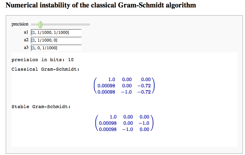
Numerical instability of the classical Gram-Schmidt algorithm
by Marshall Hampton (tested by William Stein, who thinks this is really nice!)
Linear transformations
by Jason Grout
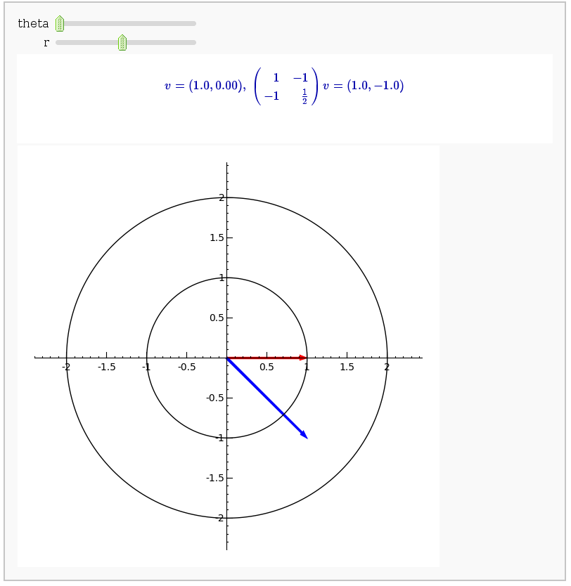
A square matrix defines a linear transformation which rotates and/or scales vectors. In the interact command below, the red vector represents the original vector (v) and the blue vector represents the image w under the linear transformation. You can change the angle and length of v by changing theta and r.
Gerschgorin Circle Theorem
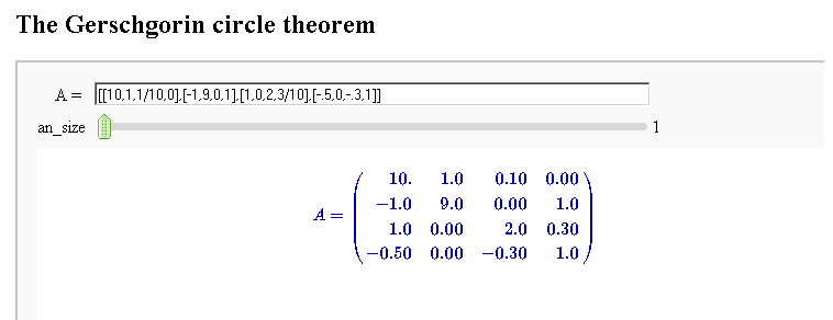
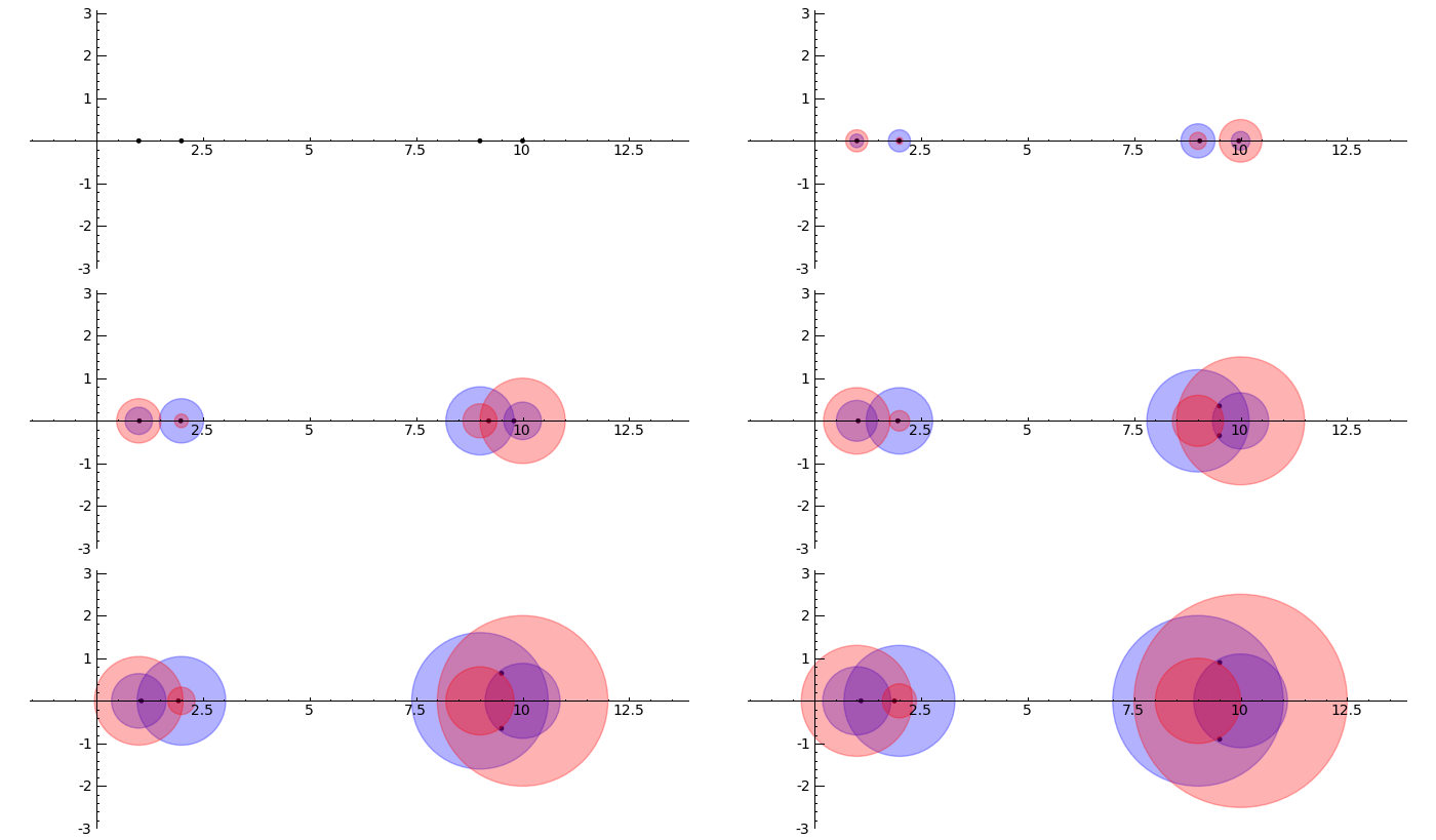
by Marshall Hampton. This animated version requires convert (imagemagick) to be installed, but it can easily be modified to a static version. The animation illustrates the idea behind the stronger version of Gerschgorin's theorem, which says that if the disks around the eigenvalues are disjoint then there is one eigenvalue per disk. The proof is by continuity of the eigenvalues under a homotopy to a diagonal matrix.
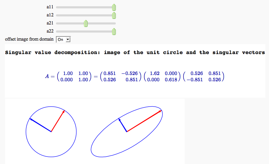
Singular value decomposition
by Marshall Hampton
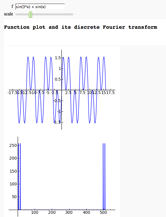
Discrete Fourier Transform
by Marshall Hampton
The Gauss-Jordan method for inverting a matrix
by Hristo Inouzhe
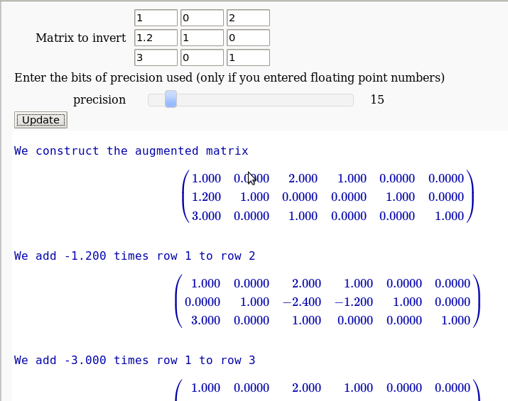
...(goes all the way to invert the matrix)
