|
Size: 18437
Comment: added Banchoff-Pohl "area"
|
← Revision 43 as of 2023-08-30 08:21:15 ⇥
Size: 18248
Comment: mini comment in Banchoff-Pohl
|
| Deletions are marked like this. | Additions are marked like this. |
| Line 6: | Line 6: |
| == Intersecting tetrahedral reflections == | == Intersecting tetrahedral reflections FIXME == |
| Line 8: | Line 8: |
| {{{ | {{{#!sagecell |
| Line 12: | Line 12: |
| p12 = p1.union(p2) | p12 = p1.convex_hull(p2) |
| Line 15: | Line 15: |
| p34 = p3.union(p4) | p34 = p3.convex_hull(p4) |
| Line 18: | Line 18: |
| p56 = p5.union(p6) | p56 = p5.convex_hull(p6) |
| Line 21: | Line 21: |
| p78 = p7.union(p8) | p78 = p7.convex_hull(p8) |
| Line 36: | Line 36: |
| {{{ | {{{#!sagecell |
| Line 52: | Line 52: |
| normal=(gammap[1]/norma(gammap), -gammap[0]/norma(gammap)) | np=norma(gammap) |
| Line 54: | Line 54: |
| np=norma(gammap) | |
| Line 57: | Line 55: |
| pe=gammap[0]*gammapp[0]+gammap[1]*gammapp[1] | normal=(gammap[1]/np, -gammap[0]/np) |
| Line 80: | Line 79: |
| show(grafica,aspect_ratio=1,xmin=-2,xmax=2,ymin=-2,ymax=2)}}} | show(grafica,aspect_ratio=1,xmin=-2,xmax=2,ymin=-2,ymax=2) }}} |
| Line 85: | Line 85: |
| by Antonio Valdés and Pablo Angulo. A first interact allows the user to introduce a parametric surface, and draws it. Then a second interact draws a geodesic within the surface. The separation is so that after the first interact, the geodesic equations are "compiled", and then the second interact is faster. {{{ u, v, t = var('u v t') @interact def _(x = input_box(3*sin(u)*cos(v), 'x'), y = input_box(sin(u)*sin(v), 'y'), z = input_box(2*cos(u), 'z'), _int_u = input_grid(1, 2, default = [[0,pi]], label = 'u -interval'), _int_v = input_grid(1, 2, default = [[-pi,pi]], label = 'v -interval')): global F, Fu, Fv, func, S_plot, int_u, int_v int_u = _int_u[0] int_v = _int_v[0] F = vector([x, y, z]) S_plot = parametric_plot3d( F, (u, int_u[0], int_u[1]), (v, int_v[0], int_v[1])) S_plot.show(aspect_ratio = [1, 1, 1]) dFu = F.diff(u) dFv = F.diff(v) Fu = fast_float(dFu, u, v) Fv = fast_float(dFv, u, v) ufunc = function('ufunc', t) vfunc = function('vfunc', t) dFtt = F(u=ufunc, v=vfunc).diff(t, t) ec1 = dFtt.dot_product(dFu(u=ufunc, v=vfunc)) ec2 = dFtt.dot_product(dFv(u=ufunc, v=vfunc)) dv, ddv, du, ddu = var('dv, ddv, du, ddu') diffec1 = ec1.subs_expr(diff(ufunc, t) == du, diff(ufunc, t, t) == ddu, diff(vfunc, t) == dv, diff(vfunc, t, t) == ddv, ufunc == u, vfunc == v) diffec2 = ec2.subs_expr(diff(ufunc, t) == du, diff(ufunc, t, t) == ddu, diff(vfunc, t) == dv, diff(vfunc, t, t) == ddv, ufunc == u, vfunc == v) sols = solve([diffec1 == 0 , diffec2 == 0], ddu, ddv) ddu_rhs = (sols[0][0]).rhs().full_simplify() ddv_rhs = (sols[0][1]).rhs().full_simplify() ddu_ff = fast_float(ddu_rhs, du, dv, u, v) ddv_ff = fast_float(ddv_rhs, du, dv, u, v) def func(y,t): v = list(y) return [ddu_ff(*v), ddv_ff(*v), v[0], v[1]] }}} {{attachment:geodesics1.png}} {{{ |
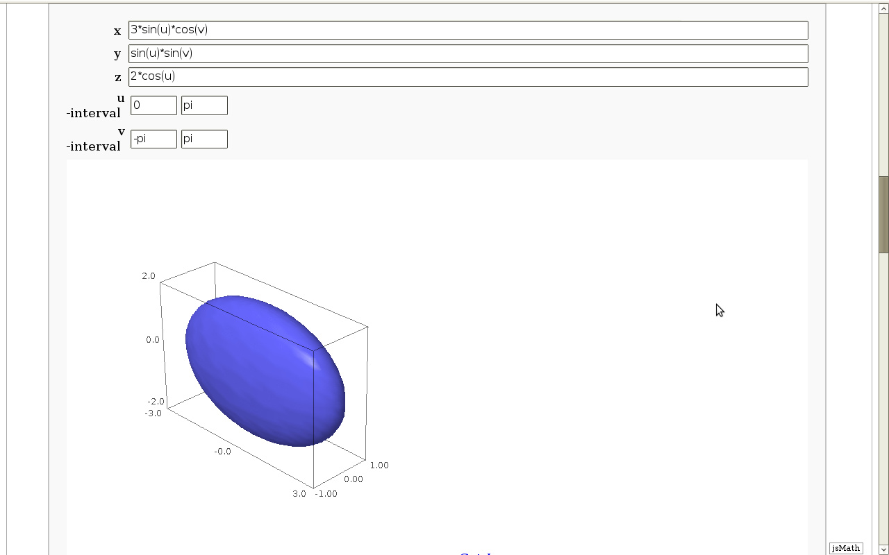
by Antonio Valdés and Pablo Angulo. This example was originally composed of two interacts: - the first allowing the user to introduce a parametric surface, and draw it. - the second drawing a geodesic within the surface. The separation was so that after the first interact, the geodesic equations were "compiled", thus making the second interact faster. However, in the following there is only one interact, to make sagecell works. {{{#!sagecell |
| Line 148: | Line 93: |
u, v, t, du, dv = var('u v t du dv') |
|
| Line 161: | Line 108: |
| def _(u_0 = slider(int_u[0], int_u[1], (int_u[1] - int_u[0])/100, default = (int_u[0] + int_u[1])/2, label = 'u_0'), v_0 = slider(int_v[0], int_v[1], (int_v[1] - int_v[0])/100, default = (int_v[0] + int_v[1])/2, label = 'v_0'), V_u = slider(-10, 10, 1/10, default = 1, label = 'V_u'), V_v = slider(-10, 10, 1/10, default = 0, label = 'V_v'), |
def _(x = input_box(3*sin(u)*cos(v), 'x'), y = input_box(sin(u)*sin(v), 'y'), z = input_box(2*cos(u), 'z'), int_u = input_grid(1, 2, default = [[0,pi]], label = 'u -interval'), int_v = input_grid(1, 2, default = [[-pi,pi]], label = 'v -interval'), init_point = input_grid(1, 2, default = [[-pi/4,pi/8]], label = 'coordinates of \ninitial point'), init_vector = input_grid(1, 2, default = [[1,0]], label = 'coordinates of \ninitial vector'), |
| Line 168: | Line 116: |
| default = (int_u[1] - int_u[0])/2, | default = pi/2, |
| Line 171: | Line 119: |
| du, dv, u, v = var('du dv u v') Point = [u_0, v_0] velocity = [V_u, V_v] Point = map(float, Point) velocity = map(float, velocity) geo2D_aux = odeint(func, y0 = [velocity[0], velocity[1], Point[0], Point[1]], t = srange(0, int_s, 0.01)) geo3D = [F(u=l,v=r) for [j, k, l, r] in geo2D_aux] if sliding_color: g_plot = fading_line3d(geo3D, rgbcolor1 = (1, 0, 0), rgbcolor2 = (0, 1, 0), thickness=4) else: g_plot = line3d(geo3D, rgbcolor=(0, 1, 0), thickness=4) P = F(u=Point[0], v=Point[1]) P_plot = point3d((P[0], P[1], P[2]), rgbcolor = (0, 0, 0), pointsize = 30) V = velocity[0] * Fu(u = Point[0], v = Point[1]) + \ velocity[1] * Fv(u= Point[0], v = Point[1]) V_plot = arrow3d(P, P + V, color = 'black') show(g_plot + S_plot + V_plot + P_plot,aspect_ratio = [1, 1, 1]) }}} |
int_u = int_u[0] int_v = int_v[0] u_0, v_0 = init_point[0] V_u, V_v = init_vector[0] F = vector([x, y, z]) S_plot = parametric_plot3d( F, (u, int_u[0], int_u[1]), (v, int_v[0], int_v[1])) dFu = F.diff(u) dFv = F.diff(v) Fu = fast_float(dFu, u, v) Fv = fast_float(dFv, u, v) ufunc = function('ufunc') vfunc = function('vfunc') dFtt = F(u=ufunc(t), v=vfunc(t)).diff(t, t) ec1 = dFtt.dot_product(dFu(u=ufunc(t), v=vfunc(t))) ec2 = dFtt.dot_product(dFv(u=ufunc(t), v=vfunc(t))) dv, ddv, du, ddu = var('dv, ddv, du, ddu') diffec1 = ec1.substitute(diff(ufunc(t), t) == du, diff(ufunc(t), t, t) == ddu, diff(vfunc(t), t) == dv, diff(vfunc(t), t, t) == ddv, ufunc(t) == u, vfunc(t) == v) diffec2 = ec2.substitute(diff(ufunc(t), t) == du, diff(ufunc(t), t, t) == ddu, diff(vfunc(t), t) == dv, diff(vfunc(t), t, t) == ddv, ufunc(t) == u, vfunc(t) == v) sols = solve([diffec1 == 0 , diffec2 == 0], ddu, ddv) ddu_rhs = (sols[0][0]).rhs().full_simplify() ddv_rhs = (sols[0][1]).rhs().full_simplify() ddu_ff = fast_float(ddu_rhs, du, dv, u, v) ddv_ff = fast_float(ddv_rhs, du, dv, u, v) def func(y,t): v = list(y) return [ddu_ff(*v), ddv_ff(*v), v[0], v[1]] Point = [u_0, v_0] velocity = [V_u, V_v] Point = list(map(float, Point)) velocity = list(map(float, velocity)) geo2D_aux = odeint(func, y0 = [velocity[0], velocity[1], Point[0], Point[1]], t = srange(0, int_s, 0.01)) geo3D = [F(u=l,v=r) for [j, k, l, r] in geo2D_aux] if sliding_color: g_plot = fading_line3d(geo3D, rgbcolor1 = (1, 0, 0), rgbcolor2 = (0, 1, 0), thickness=4) else: g_plot = line3d(geo3D, rgbcolor=(0, 1, 0), thickness=4) P = F(u=Point[0], v=Point[1]) P_plot = point3d((P[0], P[1], P[2]), rgbcolor = (0, 0, 0), pointsize = 30) V = velocity[0] * Fu(u = Point[0], v = Point[1]) + \ velocity[1] * Fv(u= Point[0], v = Point[1]) V_plot = arrow3d(P, P + V, color = 'black') show(g_plot + S_plot + V_plot + P_plot,aspect_ratio = [1, 1, 1]) }}} {{attachment:geodesics1.png}} |
| Line 203: | Line 199: |
| {{{ | {{{#!sagecell |
| Line 211: | Line 207: |
| print 'Vertices:', len(g.vertices()), ('(2^%s)'%Dimension if Calculations else ''), '\nEdges:', len(g.edges()), ('(%s*(%s/2))' %(len(g.vertices()), Dimension) if Calculations else '') | print('Vertices:', len(g.vertices()), ('(2^%s)'%Dimension if Calculations else ''), '\nEdges:', len(g.edges()), ('(%s*(%s/2))' %(len(g.vertices()), Dimension) if Calculations else '')) |
| Line 216: | Line 212: |
| print 'Vertices:', len(g.vertices()), ('(2^%s)'%Dimension if Calculations else ''), '\nEdges:', len(g.edges()), ('(%s*(%s/2))' %(len(g.vertices()), Dimension) if Calculations else '') | print('Vertices:', len(g.vertices()), ('(2^%s)'%Dimension if Calculations else ''), '\nEdges:', len(g.edges()), ('(%s*(%s/2))' %(len(g.vertices()), Dimension) if Calculations else '')) |
| Line 223: | Line 219: |
| print 'Vertices:', len(s.vertices()), ('(2^%s)'%Dimension if Calculations else ''), '\nEdges:', len(s.edges()), ('(%s*(%s/2))' %(len(s.vertices()), Dimension) if Calculations else '') | print('Vertices:', len(s.vertices()), ('(2^%s)'%Dimension if Calculations else ''), '\nEdges:', len(s.edges()), ('(%s*(%s/2))' %(len(s.vertices()), Dimension) if Calculations else '')) |
| Line 228: | Line 224: |
| print 'Vertices:', len(s.vertices()), ('(2^%s)'%Dimension if Calculations else ''), '\nEdges:', len(s.edges()), ('(%s*(%s/2))' %(len(s.vertices()), Dimension) if Calculations else '') | print('Vertices:', len(s.vertices()), ('(2^%s)'%Dimension if Calculations else ''), '\nEdges:', len(s.edges()), ('(%s*(%s/2))' %(len(s.vertices()), Dimension) if Calculations else '')) |
| Line 234: | Line 230: |
| print 'Vertices:', len(d.vertices()), ('(2^%s)'%Dimension if Calculations else ''), '\nEdges:', len(d.edges()), ('(%s*(%s/2))' %(len(d.vertices()), Dimension) if Calculations else '') | print('Vertices:', len(d.vertices()), ('(2^%s)'%Dimension if Calculations else ''), '\nEdges:', len(d.edges()), ('(%s*(%s/2))' %(len(d.vertices()), Dimension) if Calculations else '')) |
| Line 239: | Line 235: |
| print 'Vertices:', len(d.vertices()), ('(2^%s)'%Dimension if Calculations else ''), '\nEdges:', len(d.edges()), ('(%s*(%s/2))' %(len(d.vertices()), Dimension) if Calculations else '') | print('Vertices:', len(d.vertices()), ('(2^%s)'%Dimension if Calculations else ''), '\nEdges:', len(d.edges()), ('(%s*(%s/2))' %(len(d.vertices()), Dimension) if Calculations else '')) |
| Line 247: | Line 243: |
| {{{ | {{{#!sagecell |
| Line 312: | Line 308: |
| for j in xrange(partes-1)) | for j in range(partes - 1)) |
| Line 331: | Line 327: |
| print 'Number of lines with k intersection points:' print ', '.join('%d:%d'%(k,v) for k,v in d.iteritems()) |
print('Number of lines with k intersection points:') print(', '.join('%d:%d' % kv for kv in d.items())) |
| Line 334: | Line 330: |
| }}} {{{ |
|
| Line 355: | Line 349: |
| print 'A curve of lenght %f'%longitud((curvax, curvay), t0, t1) | print('A curve of length %f'%longitud((curvax, curvay), t0, t1)) |
| Line 357: | Line 351: |
| cortes_tot = sum(k*v for k,v in cortesd.iteritems()) print 'Aprox lenght using Crofton\'s formula: %f'%((cortes_tot/L)*(pi*M)) |
cortes_tot = sum(k*v for k,v in cortesd.items()) print('Approx length using Crofton\'s formula: %f'%((cortes_tot/L)*(pi*M))) |
| Line 363: | Line 357: |
| == Banchoff-Pohl area == by Pablo Angulo. Computes the Banchoff-Pohl "area enclosed by a spatial curve", by throwing some random lines and computing the linking number with the given curve. Lines not linked to the given curve are displayed in red, linked lines are displayed in green. {{{ |
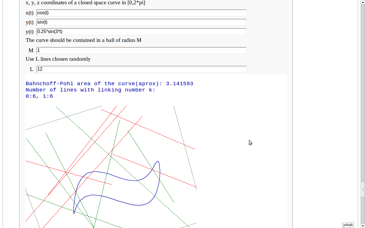
== Banchoff-Pohl "area" == by Pablo Angulo. Approximates the Banchoff-Pohl "area enclosed by a spatial curve", by throwing some random lines and computing the linking number with the given curve. Lines not linked to the given curve are displayed in red, linked lines are displayed in green. {{{#!sagecell |
| Line 416: | Line 410: |
| pp += parametric_plot3d(l1*v1+l2*v2+t*v,(t,-2,2), | # fix 30-08-23: coercion of (l1*v1+l2*v2) to SymbolicRing did not work pp += parametric_plot3d((1+0*t)*(l1*v1+l2*v2)+t*v,(t,-2,2), |
| Line 422: | Line 417: |
| print 'Number of lines with linking number k:' print ', '.join('%d:%d'%(k,v) for k,v in d.iteritems()) |
print('Number of lines with linking number k:') print(', '.join('%d:%d' % kv for kv in d.items())) |
| Line 437: | Line 432: |
| print 'Bahnchoff-Pohl area of the curve(aprox): %f'%bp_area_aprox | print('Bahnchoff-Pohl area of the curve(aprox): %f' % bp_area_aprox) |
Sage Interactions - Geometry
goto interact main page
Contents
Intersecting tetrahedral reflections FIXME
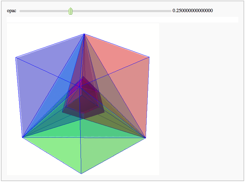
by Marshall Hampton. Inspired by a question from Hans Schepker of Glass Geometry.
Evolutes
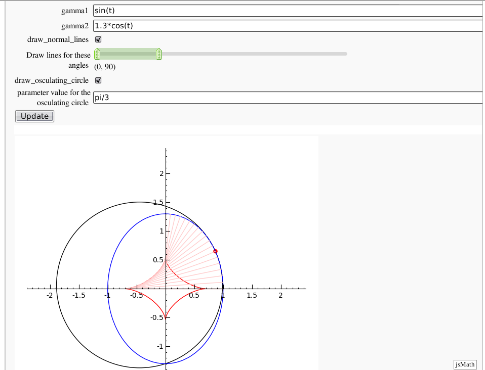
by Pablo Angulo. Computes the evolute of a plane curve given in parametric coordinates. The curve must be parametrized from the interval [0,2pi].
Geodesics on a parametric surface
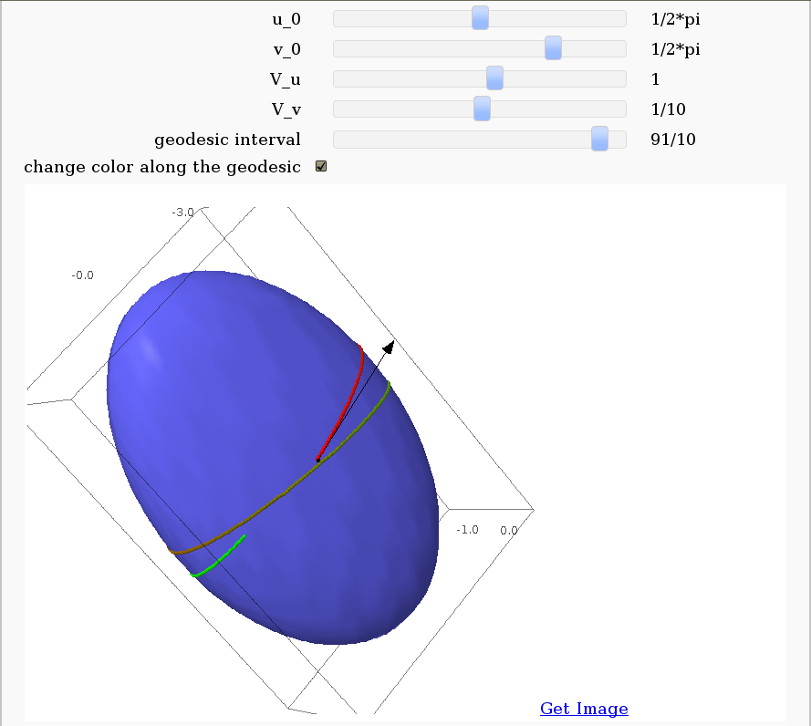
by Antonio Valdés and Pablo Angulo. This example was originally composed of two interacts:
- - the first allowing the user to introduce a parametric surface, and draw it. - the second drawing a geodesic within the surface.
The separation was so that after the first interact, the geodesic equations were "compiled", thus making the second interact faster. However, in the following there is only one interact, to make sagecell works.
Dimensional Explorer
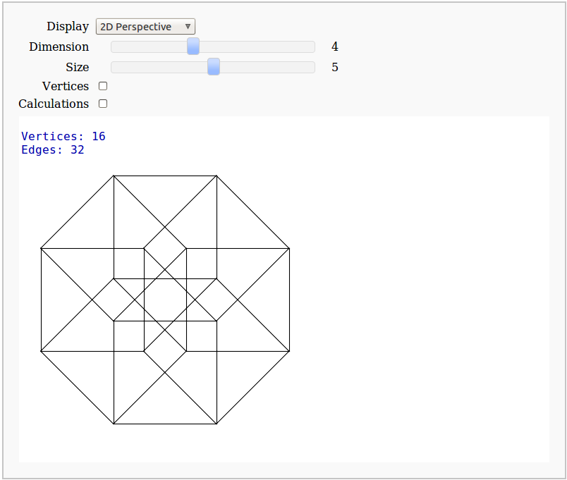
By Eviatar Bach
Renders 2D images (perspective or spring-layout) and 3D models of 0-10 dimensional hypercubes. It also displays number of edges and vertices.
Crofton's formula
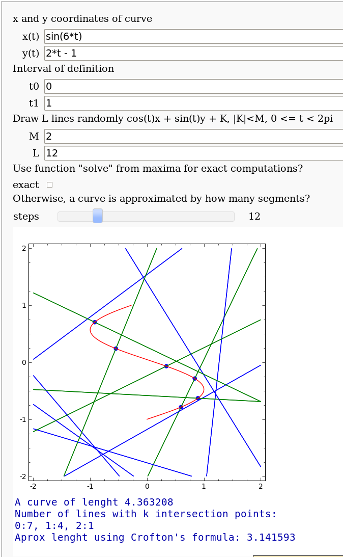
by Pablo Angulo. Illustrates Crofton's formula by throwing some random lines and computing the intersection number with a given curve. May use either solve for exact computation of the intersections, or may also approximate the curve by straight segments (this is the default).
Banchoff-Pohl "area"
by Pablo Angulo. Approximates the Banchoff-Pohl "area enclosed by a spatial curve", by throwing some random lines and computing the linking number with the given curve. Lines not linked to the given curve are displayed in red, linked lines are displayed in green.
