|
Size: 7450
Comment: Added a new interact showing geodesics on a surface
|
Size: 18327
Comment: fixing geodesics interact ...
|
| Deletions are marked like this. | Additions are marked like this. |
| Line 6: | Line 6: |
| == Intersecting tetrahedral reflections == | == Intersecting tetrahedral reflections FIXME == |
| Line 8: | Line 8: |
| {{{ | {{{#!sagecell |
| Line 12: | Line 12: |
| p12 = p1.union(p2) | p12 = p1.convex_hull(p2) |
| Line 15: | Line 15: |
| p34 = p3.union(p4) | p34 = p3.convex_hull(p4) |
| Line 18: | Line 18: |
| p56 = p5.union(p6) | p56 = p5.convex_hull(p6) |
| Line 21: | Line 21: |
| p78 = p7.union(p8) | p78 = p7.convex_hull(p8) |
| Line 36: | Line 36: |
| {{{ | {{{#!sagecell |
| Line 52: | Line 52: |
| normal=(gammap[1]/norma(gammap), -gammap[0]/norma(gammap)) | np=norma(gammap) |
| Line 54: | Line 54: |
| np=norma(gammap) | |
| Line 57: | Line 55: |
| pe=gammap[0]*gammapp[0]+gammap[1]*gammapp[1] | normal=(gammap[1]/np, -gammap[0]/np) |
| Line 80: | Line 79: |
| show(grafica,aspect_ratio=1,xmin=-2,xmax=2,ymin=-2,ymax=2)}}} | show(grafica,aspect_ratio=1,xmin=-2,xmax=2,ymin=-2,ymax=2) }}} |
| Line 85: | Line 85: |
| by Antonio Valdés and Pablo Angulo. A first interact allows the user to introduce a parametric surface, and draws it. Then a second interact draws a geodesic within the surface. The separation is so that after the first interact, the geodesic equations are "compiled", and then the second interact is faster. {{{ u, v, t = var('u v t') |
by Antonio Valdés and Pablo Angulo. This example was originally composed of two interacts: - the first allowing the user to introduce a parametric surface, and draw it. - the second drawing a geodesic within the surface. The separation was so that after the first interact, the geodesic equations were "compiled", thus making the second interact faster. This still looks as a good idea to me, so please read the original code at https://malabares.cancamusa.net/home/pub/14/ But the following is fixed so that there is only one interact, and sagecell works. There might be another way yto {{{#!sagecell from scipy.integrate import odeint u, v, t, du, dv = var('u v t du dv') def fading_line3d(points, rgbcolor1, rgbcolor2, *args, **kwds): L = len(points) vcolor1 = vector(RDF, rgbcolor1) vcolor2 = vector(RDF, rgbcolor2) return sum(line3d(points[j:j+2], rgbcolor = tuple( ((L-j)/L)*vcolor1 + (j/L)*vcolor2 ), *args, **kwds) for j in srange(L-1)) steps = 100 |
| Line 92: | Line 113: |
| _int_u = input_grid(1, 2, default = [[0,pi]], label = 'u -interval'), _int_v = input_grid(1, 2, default = [[-pi,pi]], label = 'v -interval')): global F, Fu, Fv, func, S_plot, int_u, int_v int_u = _int_u[0] int_v = _int_v[0] def F(uu, vv): X = vector([x, y, z]) return X.subs({u : uu, v : vv}) S_plot = parametric_plot3d( F(u, v), |
int_u = input_grid(1, 2, default = [[0,pi]], label = 'u -interval'), int_v = input_grid(1, 2, default = [[-pi,pi]], label = 'v -interval'), init_point = input_grid(1, 2, default = [[-pi/4,pi/8]], label = 'coordinates of \ninitial point'), init_vector = input_grid(1, 2, default = [[1,0]], label = 'coordinates of \ninitial vector'), int_s = slider(0, 10, 1/10, default = pi/2, label = 'geodesic interval'), sliding_color = checkbox(True,'change color along the geodesic')): int_u = int_u[0] int_v = int_v[0] u_0, v_0 = init_point[0] V_u, V_v = init_vector[0] F = vector([x, y, z]) S_plot = parametric_plot3d( F, |
| Line 106: | Line 132: |
| show(S_plot, aspect_ratio = [1, 1, 1]) dFu = F(u, v).diff(u) dFv = F(u, v).diff(v) |
dFu = F.diff(u) dFv = F.diff(v) |
| Line 117: | Line 142: |
| dFtt = F(ufunc, vfunc).diff(t, t) | dFtt = F(u=ufunc, v=vfunc).diff(t, t) |
| Line 138: | Line 163: |
| Line 145: | Line 170: |
| Point = [u_0, v_0] velocity = [V_u, V_v] Point = map(float, Point) velocity = map(float, velocity) geo2D_aux = odeint(func, y0 = [velocity[0], velocity[1], Point[0], Point[1]], t = srange(0, int_s, 0.01)) geo3D = [F(u=l,v=r) for [j, k, l, r] in geo2D_aux] if sliding_color: g_plot = fading_line3d(geo3D, rgbcolor1 = (1, 0, 0), rgbcolor2 = (0, 1, 0), thickness=4) else: g_plot = line3d(geo3D, rgbcolor=(0, 1, 0), thickness=4) P = F(u=Point[0], v=Point[1]) P_plot = point3d((P[0], P[1], P[2]), rgbcolor = (0, 0, 0), pointsize = 30) V = velocity[0] * Fu(u = Point[0], v = Point[1]) + \ velocity[1] * Fv(u= Point[0], v = Point[1]) V_plot = arrow3d(P, P + V, color = 'black') show(g_plot + S_plot + V_plot + P_plot,aspect_ratio = [1, 1, 1]) |
|
| Line 147: | Line 196: |
| {{{ from scipy.integrate import odeint @interact def _(u_0 = slider(int_u[0], int_u[1], default = (int_u[0] + int_u[1])/2, label = 'u_0'), v_0 = slider(int_v[0], int_v[1], default = (int_v[0] + int_v[1])/2, label = 'v_0'), V_u = slider(-10, 10, default = 1, label = 'V_u'), V_v = slider(-10, 10, default = 0, label = 'V_v'), int_s = range_slider(-10, 10, 0.1, default = (0, (int_u[1] - int_u[0])/2), label = 'geodesic interval') ): du, dv, u, v = var('du dv u v') Point = [u_0, v_0] velocity = [V_u, V_v] Point = map(float, Point) velocity = map(float, velocity) geo2D_aux = odeint(func, y0 = [velocity[0], velocity[1], Point[0], Point[1]], t = srange(int_s[0], int_s[1], 0.01)) geo3D = [F(l,r) for [j, k, l, r] in geo2D_aux] g_plot = line3d(geo3D, rgbcolor = (1, 0, 0), thickness = 4) P = F(Point[0], Point[1]) P_plot = point3d((P[0], P[1], P[2]), rgbcolor = (0, 0, 0)) V = velocity[0] * Fu(u = Point[0], v = Point[1]) + \ velocity[1] * Fv(u= Point[0], v = Point[1]) V_plot = arrow3d(P, P + V) show(g_plot + S_plot + V_plot + P_plot,aspect_ratio = [1, 1, 1]) }}} |
|
| Line 182: | Line 197: |
== Dimensional Explorer == By Eviatar Bach Renders 2D images (perspective or spring-layout) and 3D models of 0-10 dimensional hypercubes. It also displays number of edges and vertices. {{{#!sagecell @interact def render(Display=selector(['2D Perspective', '2D Spring-layout', '3D']), Dimension=slider(0,10,default=4, step_size=1), Size=slider(0,10,default=5,step_size=1), Vertices=False, Calculations=False): if Display=='2D Perspective': if Dimension==0: g=graphs.GridGraph([1]) print 'Vertices:', len(g.vertices()), ('(2^%s)'%Dimension if Calculations else ''), '\nEdges:', len(g.edges()), ('(%s*(%s/2))' %(len(g.vertices()), Dimension) if Calculations else '') g.show(figsize=[Size,Size], vertex_size=30, vertex_labels=False, transparent=True, vertex_colors='black') else: g=graphs.CubeGraph(Dimension) print 'Vertices:', len(g.vertices()), ('(2^%s)'%Dimension if Calculations else ''), '\nEdges:', len(g.edges()), ('(%s*(%s/2))' %(len(g.vertices()), Dimension) if Calculations else '') g.show(figsize=[Size,Size], vertex_size=(20 if Vertices else 0), vertex_labels=False, transparent=True, vertex_colors='black') if Display=='2D Spring-layout': if Dimension==0: s=graphs.GridGraph([1]) print 'Vertices:', len(s.vertices()), ('(2^%s)'%Dimension if Calculations else ''), '\nEdges:', len(s.edges()), ('(%s*(%s/2))' %(len(s.vertices()), Dimension) if Calculations else '') s.show(figsize=[Size,Size], vertex_size=30, vertex_labels=False, transparent=True, vertex_colors='black') else: s=graphs.GridGraph([2]*Dimension) print 'Vertices:', len(s.vertices()), ('(2^%s)'%Dimension if Calculations else ''), '\nEdges:', len(s.edges()), ('(%s*(%s/2))' %(len(s.vertices()), Dimension) if Calculations else '') s.show(figsize=[Size,Size], vertex_size=(20 if Vertices else 0), vertex_labels=False, transparent=True, vertex_colors='black') if Display=='3D': if Dimension==0: d=graphs.GridGraph([1]) print 'Vertices:', len(d.vertices()), ('(2^%s)'%Dimension if Calculations else ''), '\nEdges:', len(d.edges()), ('(%s*(%s/2))' %(len(d.vertices()), Dimension) if Calculations else '') d.show3d(figsize=[Size/2,Size/2], vertex_size=0.001) else: d=graphs.CubeGraph(Dimension) print 'Vertices:', len(d.vertices()), ('(2^%s)'%Dimension if Calculations else ''), '\nEdges:', len(d.edges()), ('(%s*(%s/2))' %(len(d.vertices()), Dimension) if Calculations else '') d.show3d(figsize=[Size,Size], vertex_size=(0.03 if Vertices else 0.001)) }}} {{attachment:dimensions.png}} == Crofton's formula == by Pablo Angulo. Illustrates [[http://en.wikipedia.org/wiki/Crofton%27s_formula| Crofton's formula]] by throwing some random lines and computing the intersection number with a given curve. May use either solve for exact computation of the intersections, or may also approximate the curve by straight segments (this is the default). {{{#!sagecell from collections import defaultdict var('t x y') pin = pi.n() def longitud(curva, t0, t1): dxdt = derivative(curva[0], t) dydt = derivative(curva[1], t) integrando(t) = sqrt(dxdt^2 + dydt^2) i,_ = numerical_integral(integrando, t0, t1) return i def random_line(cota): theta = random()*pin k = 2*cota*random() - cota return sin(theta)*x + cos(theta)*y + k def crofton_exact(curva, t0, t1, L, M): forget() assume(t>t0) assume(t<t1) pp = parametric_plot(curva, (t, t0, t1), color='red') cortesd = defaultdict(int) for k in range(L): rl = random_line(M) ss = solve(rl(x=curva[0], y=curva[1]), t) cortes = 0 for s in ss: tt = s.rhs() x0,y0 = curva[0](t=tt), curva[1](t=tt) if x0 in RR and y0 in RR: pp += point2d((x0,y0), pointsize = 30) cortes += 1 if cortes: pp += implicit_plot(rl, (x,-M,M), (y,-M,M), color='green') else: pp += implicit_plot(rl, (x,-M,M), (y,-M,M), color='blue') cortesd[cortes] += 1 return cortesd, pp def random_line_n(cota): theta = random()*pin k = 2*cota*random() - cota return sin(theta), cos(theta), k def interseccion_sr(punto1, punto2, recta): 'Devuelve el punto de interseccion de una recta y un segmento, o None si no se cortan' x1, y1 = punto1 x2, y2 = punto2 a, b, c = recta num = (-c - a*x1 - b*y1) den = (a*(x2 - x1) + b*(y2 - y1)) if (0 < num < den) or (den < num < 0): t_i = num/den return ((1-t_i)*x1 + t_i*x2, (1-t_i)*y1 + t_i*y2) else: return None def interseccion_cr(curva, t0, t1, recta, partes=50): '''Devuelve el numero de puntos de interseccion de una curva y una recta''' x,y = curva paso = (t1 - t0)/partes puntos = [(x(t=tr), y(t=tr)) for tr in srange(t0, t1 + paso, paso)] intersecciones = (interseccion_sr(puntos[j], puntos[j+1], recta) for j in xrange(partes-1)) return [p for p in intersecciones if p ] def crofton_aprox(curva, t0, t1, L, M): cortesd = defaultdict(int) pp = parametric_plot(curva, (t, t0, t1), color='red') for k in range(L): a,b,c = random_line_n(M) rl = a*x + b*y + c cortes = interseccion_cr(curva, t0, t1, (a,b,c)) if cortes: pp += sum(point2d(p, pointsize = 30) for p in cortes) pp += implicit_plot(rl, (x,-M,M), (y,-M,M), color='green') else: pp += implicit_plot(rl, (x,-M,M), (y,-M,M), color='blue') cortesd[len(cortes)] += 1 return cortesd, pp def print_stats(d): print 'Number of lines with k intersection points:' print ', '.join('%d:%d'%(k,v) for k,v in d.iteritems()) @interact def crofton_interact(u1 = text_control('x and y coordinates of curve'), curvax = input_box(t^2, label='x(t)' ), curvay = input_box(2*t-1, label='y(t)' ), u2 = text_control('Interval of definition'), t0 = 0, t1 = 1, u3 = text_control('Draw L lines randomly cos(t)x + sin(t)y + K, |K|<M, 0 <= t < 2pi'), M = 2, L = 5, u4 = text_control('Use function "solve" from maxima for exact computations?'), exact = checkbox(False), u5 = text_control('Otherwise, a curve is approximated by how many segments?'), steps = slider(4, 40, 4, 8)): if exact: cortesd, p = crofton_exact((curvax, curvay), t0, t1, L, M) else: cortesd, p = crofton_aprox((curvax, curvay), t0, t1, L, M) p.show(aspect_ratio=1, xmin=-2, xmax=2, ymin=-2,ymax=2) print 'A curve of lenght %f'%longitud((curvax, curvay), t0, t1) print_stats(cortesd) cortes_tot = sum(k*v for k,v in cortesd.iteritems()) print 'Approx length using Crofton\'s formula: %f'%((cortes_tot/L)*(pi*M)) }}} {{attachment:crofton4.png}} == Banchoff-Pohl area == by Pablo Angulo. Computes the Banchoff-Pohl "area enclosed by a spatial curve", by throwing some random lines and computing the linking number with the given curve. Lines not linked to the given curve are displayed in red, linked lines are displayed in green. {{{#!sagecell from collections import defaultdict var('t') a = 0; b= 2*pi def random_line3d(bound): '''Random line in R^3: first choose the guiding vector of the line, then choose a point in the plane p perpendicular to that vector. ''' p = vector([(2*random() - 1) for _ in range(3)]) v = p/norm(p) v2, v3 = matrix(v).right_kernel().basis() if det(matrix([v, v2, v3]))<0: v2, v3 = v3, v2 v2 = v2/norm(v2) v3 = v3 - (v3*v2)*v2 v3 = v3/norm(v3) return v, (2*random()*bound - bound, v2), (2*random()*bound - bound, v3) def winding_number(x, y, x0, y0): x -= x0 y -= y0 r2 = x^2 + y^2 xp = x.derivative(t) yp = y.derivative(t) integrando(t) = (x*yp -y*xp)/r2 i,e = numerical_integral(integrando, a, b) return round(i/(2*pi)) def linking_number(curve, line): v, (a2, v2), (a3, v3) = line M = matrix([v, v2, v3]) # curve2d = (curve*M.inverse())[1:] #This is VERY slow, for some reason! curve2d = sum(c*v for c,v in zip(curve,M.inverse()))[1:] x, y = curve2d return winding_number(x, y, a2,a3) def color_ln(number): if number: return (0,1-1/(1+number),0) else: return (1,0,0) def banchoff_pohl(curve, L, M): ln_d = defaultdict(int) pp = parametric_plot3d(curve, (t,0,2*pi), thickness=2) for k in range(L): a_line = random_line3d(M) ln = abs(linking_number(curve, a_line)) v, (l1, v1), (l2, v2) = a_line pp += parametric_plot3d(l1*v1+l2*v2+t*v,(t,-2,2), color=color_ln(ln)) ln_d[ln] += 1 return ln_d, pp def print_stats(d): print 'Number of lines with linking number k:' print ', '.join('%d:%d'%(k,v) for k,v in d.iteritems()) @interact def bp_interact( u1 = text_control('x, y, z coordinates of a closed space curve in [0,2*pi]'), curvax = input_box(cos(t), label='x(t)' ), curvay = input_box(sin(t), label='y(t)' ), curvaz = input_box(0, label='y(t)' ), u2 = text_control('The curve should be contained in a ball of radius M'), M = 1, u3 = text_control('Use L lines chosen randomly'), L = 10): ln_d, p = banchoff_pohl(vector((curvax, curvay, curvaz)), L, M) p.show(aspect_ratio=1, xmin=-2, xmax=2, ymin=-2,ymax=2) bp_area_aprox = (sum(k^2*v for k,v in ln_d.iteritems())/L)*2*pi*M^2 print 'Bahnchoff-Pohl area of the curve(aprox): %f'%bp_area_aprox print_stats(ln_d) }}} {{attachment:banchoff-pohl.png}} |
Sage Interactions - Geometry
goto interact main page
Contents
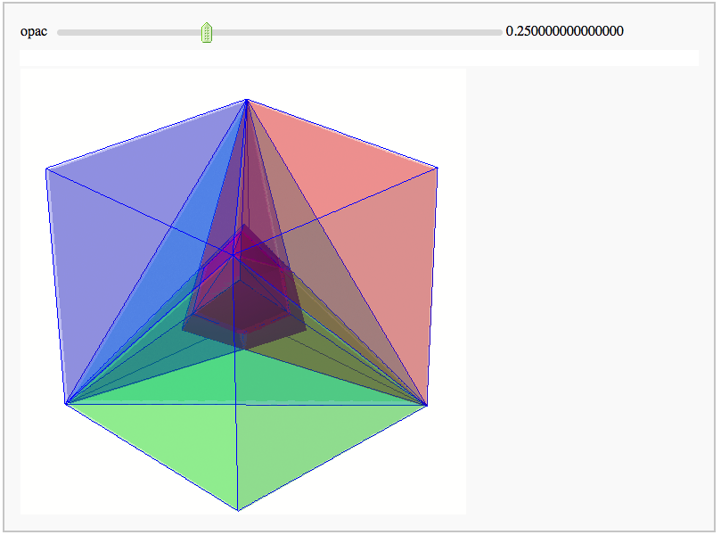
Intersecting tetrahedral reflections FIXME
by Marshall Hampton. Inspired by a question from Hans Schepker of Glass Geometry.
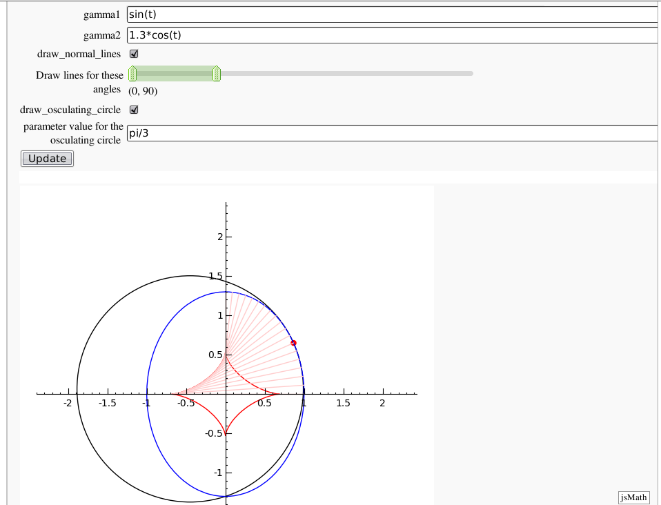
Evolutes
by Pablo Angulo. Computes the evolute of a plane curve given in parametric coordinates. The curve must be parametrized from the interval [0,2pi].
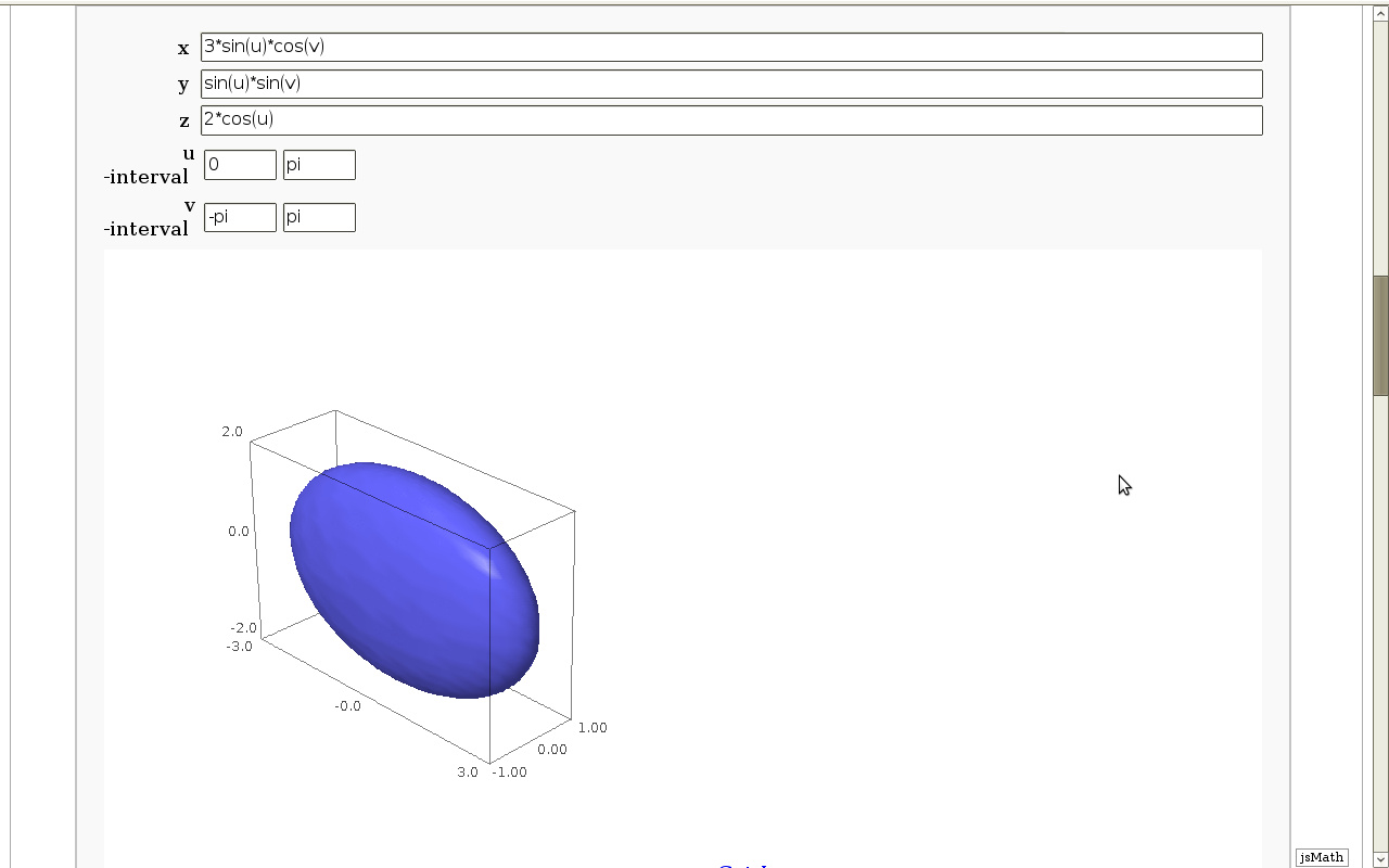
Geodesics on a parametric surface
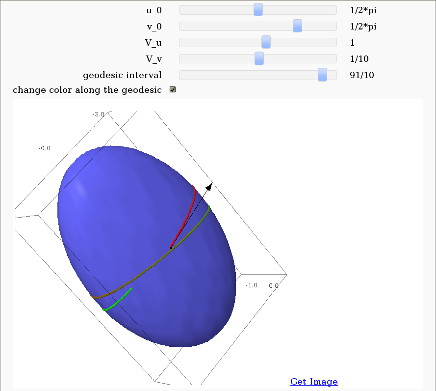
by Antonio Valdés and Pablo Angulo. This example was originally composed of two interacts:
- - the first allowing the user to introduce a parametric surface, and draw it. - the second drawing a geodesic within the surface.
The separation was so that after the first interact, the geodesic equations were "compiled", thus making the second interact faster.
This still looks as a good idea to me, so please read the original code at https://malabares.cancamusa.net/home/pub/14/ But the following is fixed so that there is only one interact, and sagecell works. There might be another way yto
Dimensional Explorer
By Eviatar Bach
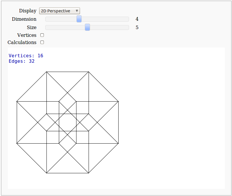
Renders 2D images (perspective or spring-layout) and 3D models of 0-10 dimensional hypercubes. It also displays number of edges and vertices.
Crofton's formula
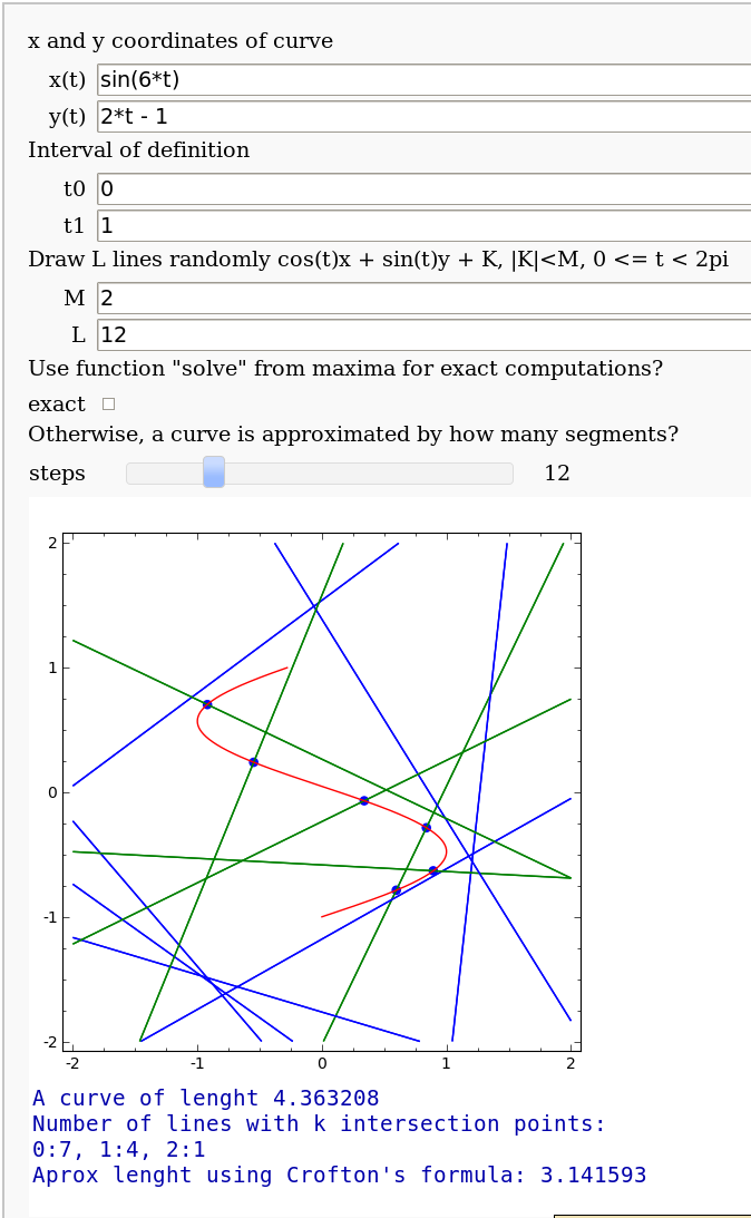
by Pablo Angulo. Illustrates Crofton's formula by throwing some random lines and computing the intersection number with a given curve. May use either solve for exact computation of the intersections, or may also approximate the curve by straight segments (this is the default).
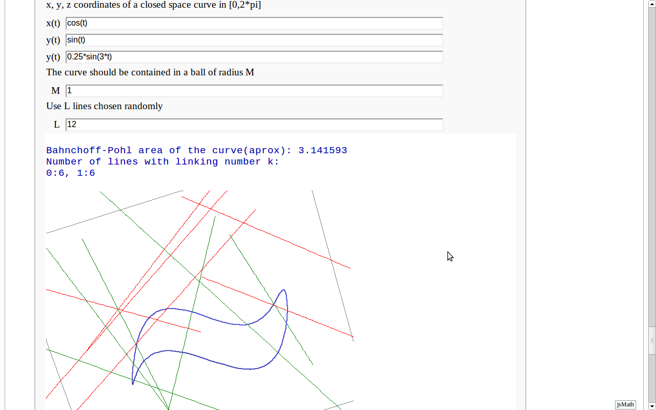
Banchoff-Pohl area
by Pablo Angulo. Computes the Banchoff-Pohl "area enclosed by a spatial curve", by throwing some random lines and computing the linking number with the given curve. Lines not linked to the given curve are displayed in red, linked lines are displayed in green.
