|
Size: 19063
Comment: fix DeprecationWarning in Linear two-dimensional ODEs
|
Size: 19066
Comment: py3 print
|
| Deletions are marked like this. | Additions are marked like this. |
| Line 450: | Line 450: |
| print 's=%f > 1/2!!! The method is not stable'%s | print('s=%f > 1/2!!! The method is not stable' % s) |
Sage Interactions - Differential Equations
goto interact main page
Contents
-
Sage Interactions - Differential Equations
- Euler's Method in one variable
- Vector Fields and Euler's Method
- Vector Field with Runga-Kutta-Fehlberg
- Linear two-dimensional ODEs
- Euler's Method, Improved Euler, and 4th order Runge-Kutta in one variable
- Mass/Spring systems
- Picard iteration example
- Euler-Maruyama method and geometric Brownian motion (a common simple model of the stock market)
- Autonomous equations and stable/unstable fixed points
- Heat equation using Fourier series
- Heat equation using finite diferences in cython
- DE with boundary values
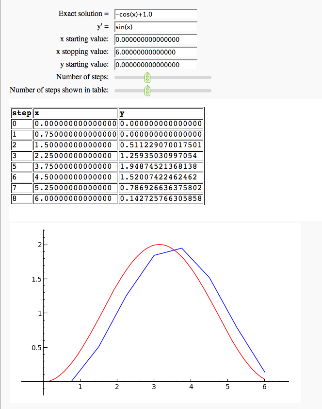
Euler's Method in one variable
by Marshall Hampton. This needs some polishing but its usable as is.
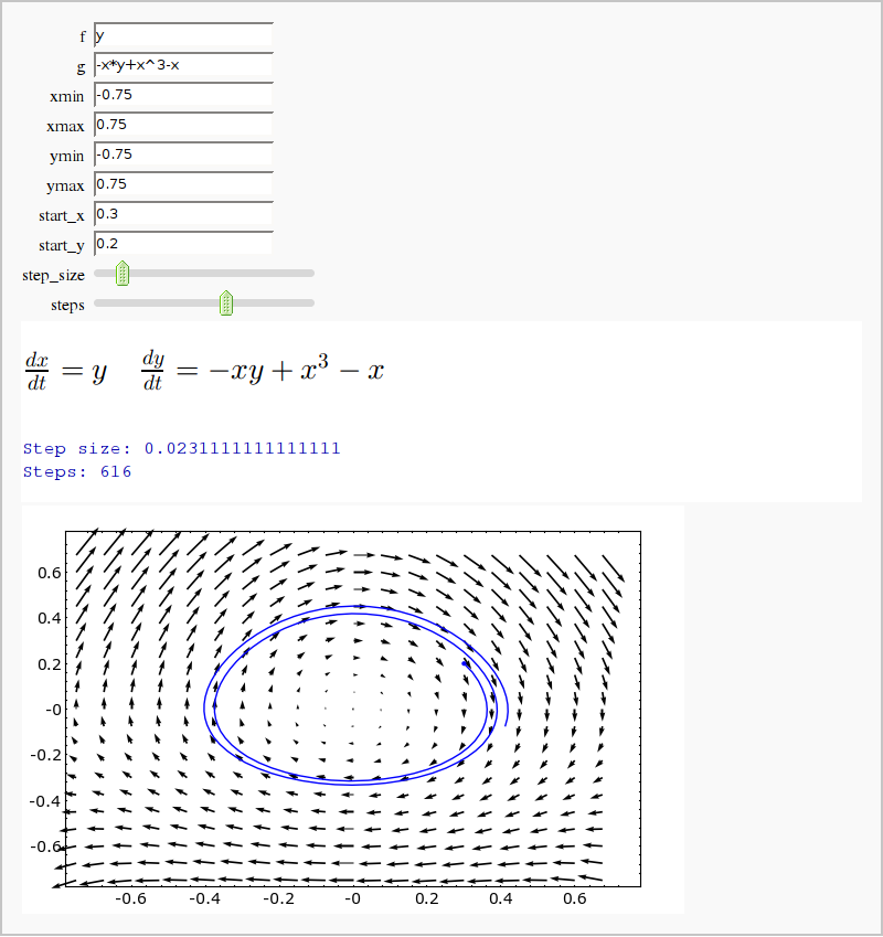
Vector Fields and Euler's Method
by Mike Hansen (tested and updated by William Stein, and later by Dan Drake)
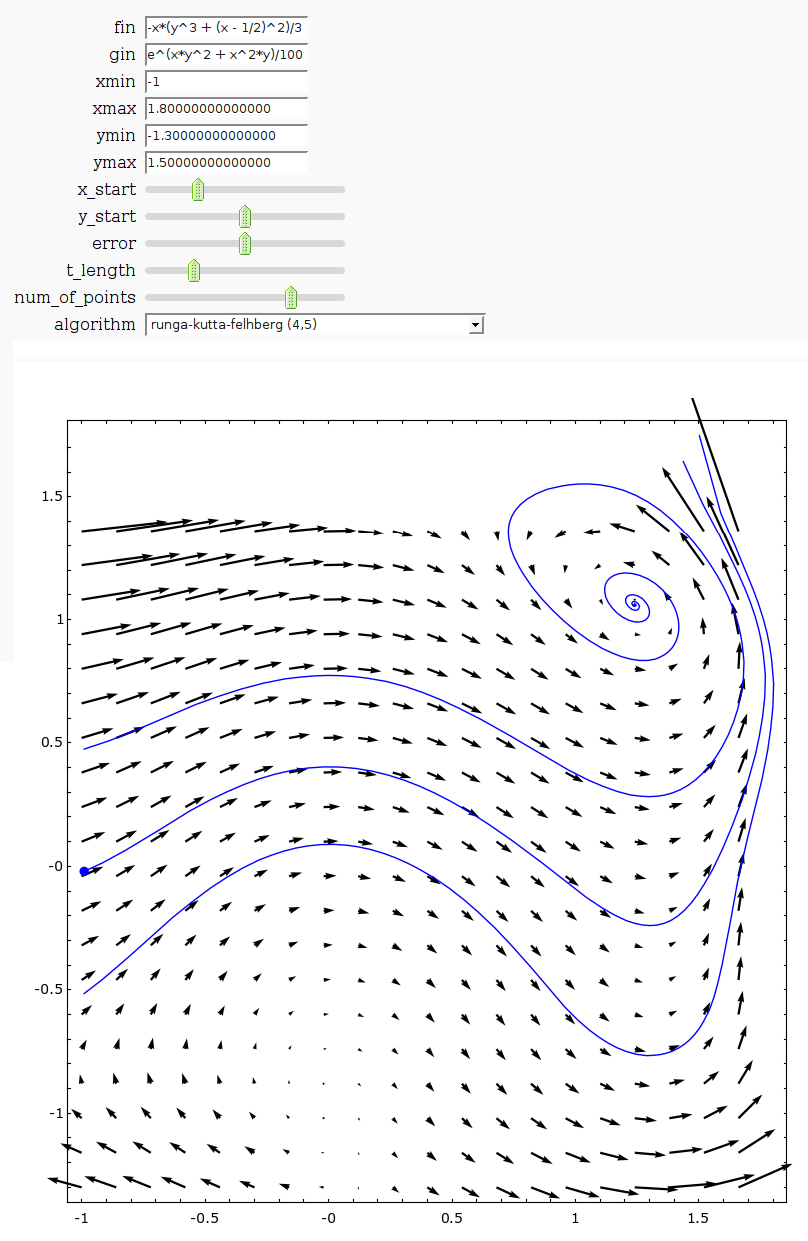
Vector Field with Runga-Kutta-Fehlberg
by Harald Schilly
Linear two-dimensional ODEs
by Marshall Hampton
%cython
cpdef c_euler_m(double t0, double x10, double x20, double tend, int steps, double a11, double a12, double a21, double a22, double cutoff = 10):
    cdef double h = (tend-t0)/steps
    traj = [[x10,x20]]
    cdef double x1current = x10
    cdef double x2current = x20
    cdef int i
    cdef double newx1
    cdef double newx2
    for i in range(0,steps):
        newx1 = x1current + h*a11*x1current + h*a12*x2current
        newx2 = x2current + h*a21*x1current + h*a22*x2current
        if newx1 > cutoff or newx2 > cutoff or newx1 < -cutoff or newx2 < -cutoff:
            break
        traj.append([newx1,newx2])
        x1current = newx1
        x2current = newx2
    return traj
@interact
def planarsystem(a11 = slider(srange(-10,10,1/10),default = -1), a12 = slider(srange(-10,10,1/10),default = -1), a21 = slider(srange(-10,10,1/10),default = 1), a22 = slider(srange(-10,10,1/10),default = -1), time_tracked = slider(srange(1,100,1.0),default=10)):
A = matrix(RDF,[[a11,a12],[a21,a22]])
eigs = A.eigenvalues()
pretty_print(html('<center>$x\' = Ax$ dynamics<BR>$A = '+latex(A)+'$, eigenvalues: $%2.2f + %2.2fI, %2.2f + %2.2fI$</center>'%(eigs[0].real(),eigs[0].imag(),eigs[1].real(),eigs[1].imag())))
trajs = Graphics()
for q in srange(0,2*pi,.15):
astart = randint(1,10)
ntraj = c_euler_m(0,cos(q),sin(q),time_tracked,300,a11,a12,a21,a22)
for i in range(astart,len(ntraj)-1,10):
trajs = trajs + arrow(ntraj[i],ntraj[i+1],width=1, arrowsize=2)
trajs = trajs + line(ntraj)
ntraj = c_euler_m(0,cos(q),sin(q),-time_tracked,300,a11,a12,a21,a22)
trajs = trajs + line(ntraj)
for i in range(astart,len(ntraj)-1,10):
trajs = trajs + arrow(ntraj[i+1],ntraj[i],width=1, arrowsize=2)
show(trajs, figsize = [6,6], xmin = -1, xmax = 1, ymin = -1, ymax = 1)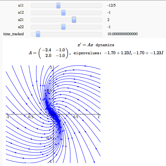
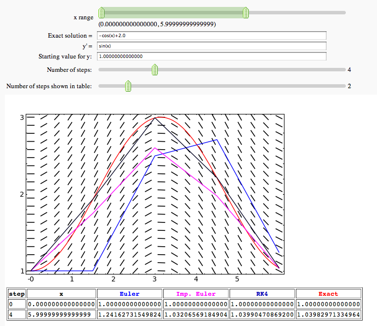
Euler's Method, Improved Euler, and 4th order Runge-Kutta in one variable
by Marshall Hampton. This is a more baroque version of the Euler's method demo above.
Mass/Spring systems
by Jason Grout
These two interacts involve some Cython code or other scipy imports, so I've posted a file containing them. You can download the worksheet or copy it online.
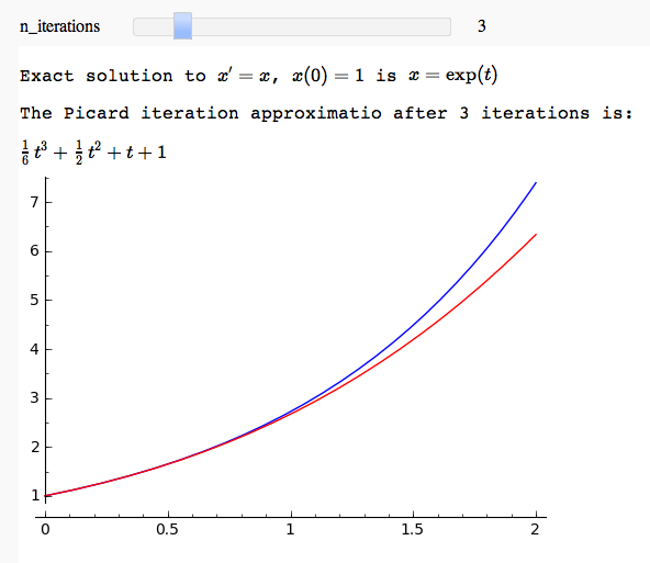
Picard iteration example
by Marshall Hampton and David Joyner
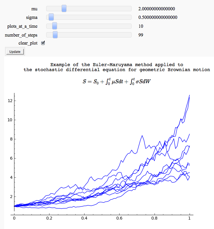
Euler-Maruyama method and geometric Brownian motion (a common simple model of the stock market)
by Marshall Hampton
Autonomous equations and stable/unstable fixed points
by Marshall Hampton This needs the Cython functon defined in a seperate cell. Note that it is not a particularly good example of Cython use.
%cython
cpdef RK4_1d(f, double t_start, double y_start, double t_end, int steps, double y_upper = 10**6, double y_lower = -10**6):
    '''
    Fourth-order scalar Runge-Kutta solver with fixed time steps. f must be a function of t,y,
    where y is just a scalar variable.
    '''
    cdef double step_size = (t_end - t_start)/steps
    cdef double t_current = t_start
    cdef double y_current = y_start
    cdef list answer_table = []
    cdef int j
    answer_table.append([t_current,y_current])
    for j in range(0,steps):
        k1=f(t_current, y_current)
        k2=f(t_current+step_size/2, y_current + k1*step_size/2)
        k3=f(t_current+step_size/2, y_current + k2*step_size/2)
        k4=f(t_current+step_size, y_current + k3*step_size)
        t_current += step_size
        y_current = y_current + (step_size/6)*(k1+2*k2+2*k3+k4)
        if y_current > y_upper or y_current < y_lower:
            j = steps
        answer_table.append([t_current,y_current])
    return answer_table
from sage.rings.polynomial.real_roots import *
var('x')
@interact
def autonomous_plot(poly=input_box(x*(x-1)*(x-2),label='polynomial'), t_end = slider(1,10,step_size = .1)):
var('x')
y = polygen(ZZ)
ypoly = sage_eval(repr(poly).replace('x','y'),locals=locals())
rr = real_roots(ypoly, max_diameter = 1/100)
eps = 0.2
delvals = .04
minr = min([x[0][0] for x in rr])
maxr = max([x[0][1] for x in rr])
svals = [(minr-eps)*t+(1-t)*(maxr+eps) for t in srange(0,1+delvals,delvals)]
def polyf(t,xi):
return poly(x=xi)
paths = [RK4_1d(polyf,0.0,q,t_end,100.0) for q in svals]
miny = max(minr-eps,min([min([q1[1] for q1 in q]) for q in paths]))
maxy = min(maxr+eps,max([max([q1[1] for q1 in q]) for q in paths]))
solpaths = sum([line(q) for q in paths])
fixedpoints = sum([line([[0,(q[0][0]+q[0][1])/2],[t_end,(q[0][0]+q[0][1])/2]], rgbcolor = (1,0,0)) for q in rr])
var('t')
html("Autonomous differential equation $x' = p(x)$")
show(solpaths+fixedpoints, ymin = miny, ymax = maxy, xmin = 0, xmax = t_end, figsize = [6,4])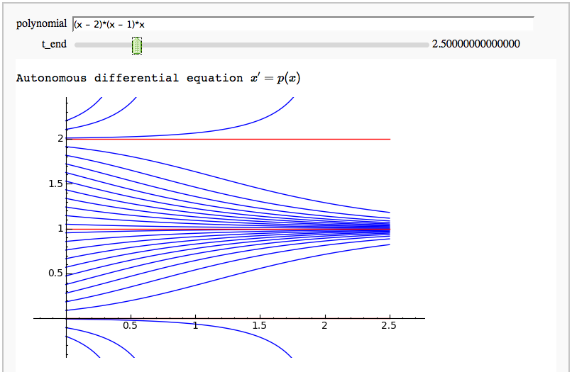
Heat equation using Fourier series
by Pablo Angulo
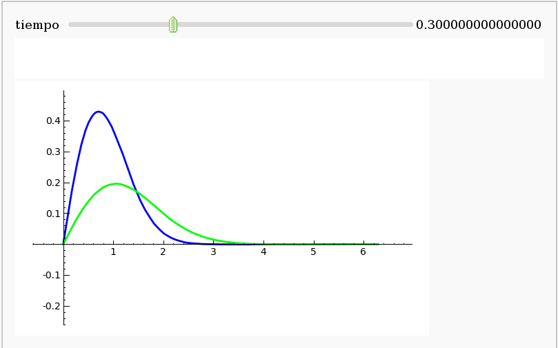
Heat equation using finite diferences in cython
by Pablo Angulo
%cython
#cython code implementing a very simple finite diference scheme
import numpy as np
def calor_cython(u0,float dx, float k,float t_f,int tsteps):
    cdef int m
    cdef float dt
    cdef float s
    u=np.array(u0)
    dt=t_f/tsteps
    s=k*dt/(dx**2)        #we cannot use ^ for exponentiation in cython
    for m in range(tsteps):
        u[1:-1]=(1-2*s)*u[1:-1]+s*u[0:-2]+s*u[2:]
    return u
#interact box wrapping the code above
var('x')
@interact
def _(f=input_box(default=x*exp(-x^2),label='f(x)'), longitud=input_box(default=2*pi),
tiempo=input_box(default=0.1), M=input_box(default=100),
k=input_box(default=1), tsteps=input_box(default=2000) ):
efe=f._fast_float_(x)
dx=float(longitud/M)
xs=[n*dx for n in range(M+1)]
u0=[efe(a) for a in xs]
s=k*(tiempo/tsteps) /dx^2
if s>0.5:
print('s=%f > 1/2!!! The method is not stable' % s)
ut=calor_cython(u0,dx,k,tiempo,tsteps)
show( line2d(zip(xs, u0)) + line2d(zip(xs, ut), rgbcolor='green') )
DE with boundary values
The following interact demo looks at the DE+BC y'+y=0, y(0)=a, y(b)=c, and has a slider for b. When b=pi "problems arise":-)
