|
Size: 10736
Comment:
|
Size: 13965
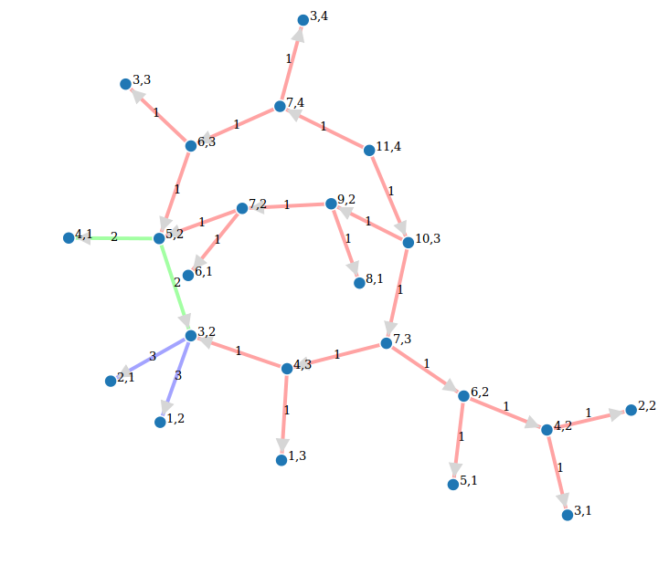
Comment: D3js interactive version of Call graph of a recursive function
|
| Deletions are marked like this. | Additions are marked like this. |
| Line 205: | Line 205: |
| === Three famous plots of chaos === | === Feigenbaum diagram === Author: Pablo Angulo Posted to sage-devel 2008-09-13. See also https://sage.math.washington.edu:8101/home/pub/3 #Note: Mandelbrot set moved to interact/fractals |
| Line 207: | Line 211: |
| # Author: Pablo Angulo Posted to sage-devel 2008-09-13. See also https://sage.math.washington.edu:8101/home/pub/3 ----------------------------------- |
|
| Line 232: | Line 231: |
--------------------------------------- #Lorentz attractor #plots the orbit of the point (1,1,1) using the simplest euler method h=0.01; # time step k=2000 # number of iterations (time k*h will be reached) sigma=10; #parameters rho=28; beta=8/3; x=1; y=1; z=1; # initial data puntos=[] for i in range(k): x,y,z=x+h*( sigma*(y-x) ), y+h*( x*(rho - z) - y ), z+h*( x*y - beta*z ) puntos.append((x,y,z)) point3d(puntos) -------------------------------------------- #Mandelbrot set: the final plot is a subset of the complex plane; #the color at point c is proportional to the number of iterations that #the discrete dynamical system z->z^2+c takes to leave a circle around #the origin when z0=0 N=100 #resolution of the plot L=50 #limits the number of iterations x0=-2; x1=1; y0=-1.5; y1=1.5 #boundary of the region plotted R=3 #stop after leaving the circle of radius R m=matrix(N,N) for i in range(N): for k in range(N): c=complex(x0+i*(x1-x0)/N, y0+k*(y1-y0)/N) z=0 h=0 while h<L and abs(z)<R: z=z*z+c h+=1 m[i,k]=h matrix_plot(m) }}} |
}}} |
| Line 278: | Line 234: |
| {{attachment:mandelbrot1.png}} | |
| Line 324: | Line 279: |
=== Integral Curvature Apollonian Circle Packing === by Marshall Hampton and Carl Witty {{{ def kfun(k1,k2,k3,k4): """ The Descartes formula for the curvature of an inverted tangent circle. """ return 2*k1+2*k2+2*k3-k4 colorlist = [(1,0,1),(0,1,0),(0,0,1),(1,0,0)] def circfun(c1,c2,c3,c4): """ Computes the inversion of circle 4 in the first three circles. """ newk = kfun(c1[3],c2[3],c3[3],c4[3]) newx = (2*c1[0]*c1[3]+2*c2[0]*c2[3]+2*c3[0]*c3[3]-c4[0]*c4[3])/newk newy = (2*c1[1]*c1[3]+2*c2[1]*c2[3]+2*c3[1]*c3[3]-c4[1]*c4[3])/newk newcolor = c4[4] if newk > 0: newr = 1/newk elif newk < 0: newr = -1/newk else: newr = Infinity return [newx, newy, newr, newk, newcolor] def mcircle(circdata, label = False, thick = 1/10, cutoff = 2000, color = ''): """ Draws a circle from the data. label = True """ if color == '': color = colorlist[circdata[4]] if label==True and circdata[3] > 0 and circdata[2] > 1/cutoff: lab = text(str(circdata[3]),(circdata[0],circdata[1]), fontsize = \ 500*(circdata[2])^(.95), vertical_alignment = 'center', horizontal_alignment \ = 'center', rgbcolor = (0,0,0),zorder=10) else: lab = Graphics() circ = circle((circdata[0],circdata[1]), circdata[2], rgbcolor = (0,0,0), \ thickness = thick) circ = circ + circle((circdata[0],circdata[1]), circdata[2], rgbcolor = color, \ thickness = thick, fill=True, alpha = .4, zorder=0) return lab+circ def add_circs(c1, c2, c3, c4, cutoff = 300): """ Find the inversion of c4 through c1,c2,c3. Add the result to circlist, then (if the result is big enough) recurse. """ newcirc = circfun(c1, c2, c3, c4) if newcirc[3] < cutoff: circlist.append(newcirc) add_circs(newcirc, c1, c2, c3, cutoff = cutoff) add_circs(newcirc, c2, c3, c1, cutoff = cutoff) add_circs(newcirc, c3, c1, c2, cutoff = cutoff) zst1 = [0,0,1/2,-2,0] zst2 = [1/6,0,1/3,3,1] zst3 = [-1/3,0,1/6,6,2] zst4 = [-3/14,2/7,1/7,7,3] circlist = [zst1,zst2,zst3,zst4] add_circs(zst1,zst2,zst3,zst4,cutoff = 500) add_circs(zst2,zst3,zst4,zst1,cutoff = 500) add_circs(zst3,zst4,zst1,zst2,cutoff = 500) add_circs(zst4,zst1,zst2,zst3,cutoff = 500) circs = sum([mcircle(q, label = True, thick = 1/2) for q in \ circlist[1:]]) circs = circs + mcircle(circlist[0],color=(1,1,1),thick=1) circs.save('./Apollonian3.png',axes = False, figsize = [12,12], xmin = \ -1/2, xmax = 1/2, ymin = -1/2, ymax = 1/2) }}} {{attachment:Apollonian.png}} === Call graph of a recursive function === {{{ def grafo_llamadas(f): class G(object): def __init__(self, f): self.f=f self.stack = [] self.g = DiGraph() def __call__(self, *args): if self.stack: sargs = ','.join(str(a) for a in args) last = ','.join(str(a) for a in self.stack[-1]) if self.g.has_edge(last, sargs): l = self.g.edge_label(last, sargs) self.g.set_edge_label(last, sargs, l + 1) else: self.g.add_edge(last, sargs, 1) else: self.g = DiGraph() self.stack.append(args) v = self.f(*args) self.stack.pop() return v def grafo(self): return self.g return G(f) @grafo_llamadas def particiones(n, k): if k == n: return [[1]*n] if k == 1: return [[n]] if not(0 < k < n): return [] ls1 = [p+[1] for p in particiones(n-1, k-1)] ls2 = [[parte+1 for parte in p] for p in particiones(n-k, k)] return ls1 + ls2 particiones(13,5) g = particiones.grafo() g.show(edge_labels=True, figsize=(6,6), vertex_size=500, color_by_label=True) }}} {{{#D3js interactive version (just a screenshot here) edge_partition = [ [edge for edge in g.edges() if edge[-1]==el] for el in set(g.edge_labels()) ] g.show(method='js', edge_labels=True, vertex_labels=True, link_distance=90, charge=-400, link_strength=2, force_spring_layout=True, edge_partition=edge_partition) }}} {{attachment:call_graph_partitions_js_2.png}} {{attachment:call_graph_partitions.png}} |
Pictures drawn by Sage
These pictures and images were drawn by Sage.
Contents
-
Pictures drawn by Sage
- Everywhere continuous, nowhere differentiable function
- Mirrored balls in tachyon
- Math art by Tom Boothby
- Twisted cubic in tachyon
- Reflections from four spheres in tachyon
- A cone inside a sphere
- A cylinder inside a cone
- A hypotrochoid animation by Dean Moore
- A simpler hypotrochoid
- The witch of Maria Agnesi
- p-adic Seasons Greetings
- Lorentz butterfly
- Feigenbaum diagram
- Sierpinski triangle
- The Tamer and the Lion by Provencal and Labbe
- Integral Curvature Apollonian Circle Packing
- Call graph of a recursive function
Everywhere continuous, nowhere differentiable function
- Everywhere continuous, nowhere differentiable function (in the infinite limit, anyway):
p = Graphics()
for n in range(1,20):
  f = lambda x: sum([sin(x*3^i)/(2^i) for i in range(1,n)])
  p += plot(f,0,float(pi/3),plot_points=2000,rgbcolor=hue(n/20))

p.show(xmin=0, ymin=0,dpi=250)

Mirrored balls in tachyon
t = Tachyon(camera_center=(8.5,5,5.5), look_at=(2,0,0), raydepth=6, xres=1500, yres=1500)
t.light((10,3,4), 1, (1,1,1))
t.texture('mirror', ambient=0.05, diffuse=0.05, specular=.9, opacity=0.9, color=(.8,.8,.8))
t.texture('grey', color=(.8,.8,.8), texfunc=7) ## try other values of texfunc too!
t.plane((0,0,0),(0,0,1),'grey')
t.sphere((4,-1,1), 1, 'mirror')
t.sphere((0,-1,1), 1, 'mirror')
t.sphere((2,-1,1), 0.5, 'mirror')
t.sphere((2,1,1), 0.5, 'mirror')
show(t)

Math art by Tom Boothby
# Author: Tom Boothby
# This is a remake of an old art piece I made in POVRay


t = Tachyon(xres=1000,yres=600, camera_center=(1,0,5), antialiasing=3)
t.light((4,3,2), 0.2, (1,1,1))
t.texture('t0', ambient=0.1, diffuse=0.9, specular=0.5, opacity=1.0, color=(1.0,1,1))
t.texture('t1', ambient=0.5, diffuse=0.5, specular=0.0, opacity=1.0, color=(0,0,0))
t.texture('t2', ambient=0.2, diffuse=0.7, specular=0, opacity=0.7, color=(.5,.5,.5))
t.texture('t3', ambient=.9, diffuse=5, specular=0,opacity=.1, color=(1,0,0))
t.sphere((1,0,0), 30, 't2')


k=0
for i in srange(-pi*10,0,.01):
  k += 1
  t.sphere((cos(i/10)-.1, sin(i/10)*cos(i), sin(i/10)*sin(i)), 0.1, 't0')
  t.sphere((cos(i/10) + 2.1, sin(i/10)*cos(i), sin(i/10)*sin(i)), 0.1, 't1')

t.show(verbose=1)

Twisted cubic in tachyon
t = Tachyon(xres=512,yres=512, camera_center=(5,0,0))
t.light((4,3,2), 0.2, (1,1,1))
t.texture('t0', ambient=0.1, diffuse=0.9, specular=0.5, opacity=1.0, color=(1.0,0,0))
t.texture('t1', ambient=0.1, diffuse=0.9, specular=0.3, opacity=1.0, color=(0,1.0,0))
t.texture('t2', ambient=0.2, diffuse=0.7, specular=0.5, opacity=0.7, color=(0,0,1.0))
k=0
for i in srange(-5,1.5,0.1):
    k += 1
    t.sphere((i,i^2-0.5,i^3), 0.1, 't%s'%(k%3))

t.show()

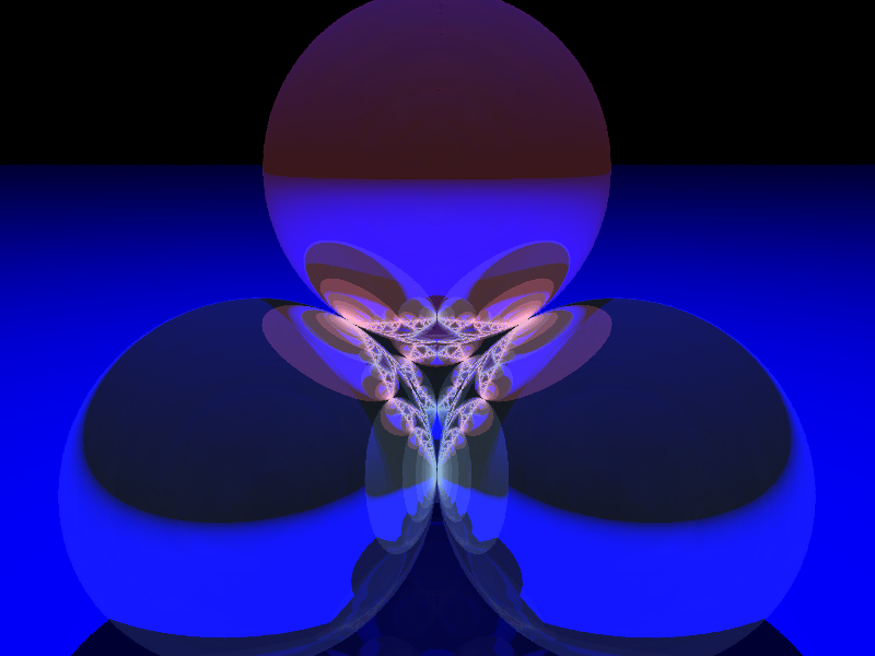
Reflections from four spheres in tachyon
t6 = Tachyon(camera_center=(0,-4,1), xres = 800, yres = 600, raydepth = 12, aspectratio=.75, antialiasing = True)
t6.light((0.02,0.012,0.001), 0.01, (1,0,0))
t6.light((0,0,10), 0.01, (0,0,1))
t6.texture('s', color = (.8,1,1), opacity = .9, specular = .95, diffuse = .3, ambient = 0.05)
t6.texture('p', color = (0,0,1), opacity = 1, specular = .2)
t6.sphere((-1,-.57735,-0.7071),1,'s')
t6.sphere((1,-.57735,-0.7071),1,'s')
t6.sphere((0,1.15465,-0.7071),1,'s')
t6.sphere((0,0,0.9259),1,'s')
t6.plane((0,0,-1.9259),(0,0,1),'p')
t6.show()
A cone inside a sphere
sage: u,v = var("u,v")
sage: p1 = parametric_plot3d([cos(u)*v, sin(u)*v, 3*v/2-1/3], (u, 0, 2*pi), (v, 0, 0.95),plot_points=[20,20])
sage: p2 = sphere((0,0,2/3), color='red', opacity=0.5, aspect_ratio=[1,1,1])
sage: show(p1+p2)

A cylinder inside a cone
sage: u,v = var("u,v")
sage: p1 = parametric_plot3d([cos(u)*v, sin(u)*v, 3/2-3*v/2], (u, 0, 2*pi), (v, 0, 1.5), opacity = 0.5, plot_points=[20,20])
sage: p2 = parametric_plot3d([cos(u)/2, sin(u)/2, v-3/4], (u, 0, 2*pi), (v, 0, 3/2), plot_points=[20,20])
sage: show(p1+p2)

A hypotrochoid animation by Dean Moore
Hypotrochoid. Written by Dean Moore, February 2008
This animation was moved to the section on the animate command : http://wiki.sagemath.org/animate#AhypotrochoidanimationbyDeanMoore
A simpler hypotrochoid
This animation was moved to the section on the animate command : http://wiki.sagemath.org/animate#Asimplerhypotrochoid
The witch of Maria Agnesi
by Marshall Hampton
This animation was moved to the section on the animate command : http://wiki.sagemath.org/animate#ThewitchofMariaAgnesi
p-adic Seasons Greetings
- I know this is early, but thanks to Robert Bradshaw's p-adic plot function, here is a p-adic Seasons Greetings:

This is the code:
sage: P1 = Zp(3).plot(rgbcolor=(0,1,0))
sage: P2 = Zp(7).plot(rgbcolor=(1,0,0))
sage: P3 = text("$Seasons$ $Greetings$ ",(0.0,1.8))
sage: P4 = text("$from$ $everyone$ $at$ sagemath.org!",(0.1,-1.6))
sage: (P1+P2+P3+P4).show(axes=False)
Lorentz butterfly
"""
Draws Loretz butterfly using matplotlib (2d) or jmol (3d).
Written by Matthew Miller and William Stein.

"""

def butterfly2d():
    """"
    EXAMPLE:
        sage: butterfly2d()
    """
    g = Graphics()
    x1, y1 = 0, 0
    from math import sin, cos, exp, pi
    for theta in srange( 0, 10*pi, 0.01 ):
        r = exp(cos(theta)) - 2*cos(4*theta) + sin(theta/12)^5
        x = r * cos(theta)  # Convert polar to rectangular coordinates
        y = r * sin(theta)
        xx = x*6 + 25       # Scale factors to enlarge and center the curve.
        yy = y*6 + 25
        if theta != 0:
            l = line( [(x1, y1), (xx, yy)], rgbcolor=hue(theta/7 + 4) )
            g = g + l
            x1, y1 = xx, yy
    g.show(dpi=100, axes=False)

def butterfly3d():
    """"
    EXAMPLE:
        sage: butterfly3d()
    """
    g = point3d((0,0,0))
    x1, y1 = 0, 0
    from math import sin, cos, exp, pi
    for theta in srange( 0, 10*pi, 0.05):
        r = exp(cos(theta)) - 2*cos(4*theta) + sin(theta/12)^5
        x = r * cos(theta)  # Convert polar to rectangular coordinates
        y = r * sin(theta)
        xx = x*6 + 25       # Scale factors to enlarge and center the curve.
        yy = y*6 + 25
        if theta != 0:
            l = line3d( [(x1, y1, theta), (xx, yy, theta)],
            rgbcolor=hue(theta/7 + 4) )
            g = g + l
            x1, y1 = xx, yy
    g.show(dpi=100, axes=False)


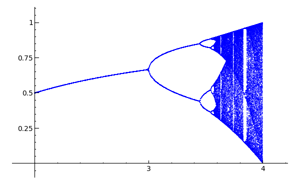
Feigenbaum diagram
Author: Pablo Angulo Posted to sage-devel 2008-09-13. See also https://sage.math.washington.edu:8101/home/pub/3 #Note: Mandelbrot set moved to interact/fractals
#Plots Feigenbaum diagram: divides the parameter interval [2,4] for mu
#into N steps. For each value of the parameter, iterate the discrete
#dynamical system x->mu*x*(1-x), drop the first M1 points in the orbit
#and plot the next M2 points in a (mu,x) diagram

N=200
M1=200
M2=200
x0=0.509434

puntos=[]
for t in range(N):
   mu=2.0+2.0*t/N
   x=x0
   for i in range(M1):
       x=mu*x*(1-x)
   for i in range(M2):
       x=mu*x*(1-x)
       puntos.append((mu,x))
point(puntos,pointsize=1)
Sierpinski triangle
- This was a black+white Sierpinski triangle coded by Marshall Hampton, with some slight tweeking by David Joyner to add colors:
def sierpinski_seasons_greetings():
    """
    Code by Marshall Hampton.
    Colors by David Joyner.
    General depth by Rob Beezer.
    Copyright Marshall Hampton 2008, licensed
    creative commons, attribution share-alike.
    """
    depth = 7
    nsq = RR(3^(1/2))/2.0
    tlist_old = [[[-1/2.0,0.0],[1/2.0,0.0],[0.0,nsq]]]
    tlist_new = tlist_old[:]
    for ind in range(depth):
       for tri in tlist_old:
           for p in tri:
               new_tri = [[(p[0]+x[0])/2.0, (p[1]+x[1])/2.0] for x in tri]
               tlist_new.append(new_tri)
       tlist_old = tlist_new[:]
    T = tlist_old
    N  = 4^depth
    N1 = N - 3^depth
    q1 = sum([line(T[i]+[T[i][0]], rgbcolor = (0,1,0)) for i in range(N1)])
    q2 = sum([line(T[i]+[T[i][0]], rgbcolor = (1,0,0)) for i in range(N1,N)])
    show(q2+q1, figsize = [6,6*nsq], axes = False)
GIMP was used to add a Season's greetings message:

Also (thanks to Rob Beezer) available in poster form in pdf format: http://sage.math.washington.edu/home/wdj/art/seasons-greetings-sage.pdf, and in A4 size: http://sage.math.washington.edu/home/wdj/art/seasons-greetings-sage-a4.pdf.
The Tamer and the Lion by Provencal and Labbe
This animation was moved to the section on the animate command : http://wiki.sagemath.org/animate#TheTamerandtheLionbyProvencalandLabbe
Integral Curvature Apollonian Circle Packing
by Marshall Hampton and Carl Witty
def kfun(k1,k2,k3,k4):
    """
    The Descartes formula for the curvature of an inverted tangent circle.
    """
    return 2*k1+2*k2+2*k3-k4


colorlist = [(1,0,1),(0,1,0),(0,0,1),(1,0,0)]

def circfun(c1,c2,c3,c4):
    """
    Computes the inversion of circle 4 in the first three circles.
    """
    newk = kfun(c1[3],c2[3],c3[3],c4[3])
    newx = (2*c1[0]*c1[3]+2*c2[0]*c2[3]+2*c3[0]*c3[3]-c4[0]*c4[3])/newk
    newy = (2*c1[1]*c1[3]+2*c2[1]*c2[3]+2*c3[1]*c3[3]-c4[1]*c4[3])/newk
    newcolor = c4[4]
    if newk > 0:
        newr = 1/newk
    elif newk < 0:
        newr = -1/newk
    else:
        newr = Infinity
    return [newx, newy, newr, newk, newcolor]

def mcircle(circdata, label = False, thick = 1/10, cutoff = 2000, color = ''):
    """
    Draws a circle from the data.  label = True
    """
    if color == '':
        color = colorlist[circdata[4]]
    if label==True and circdata[3] > 0 and circdata[2] > 1/cutoff:
        lab = text(str(circdata[3]),(circdata[0],circdata[1]), fontsize = \
500*(circdata[2])^(.95), vertical_alignment = 'center', horizontal_alignment \
= 'center', rgbcolor = (0,0,0),zorder=10)
    else:
        lab = Graphics()
    circ = circle((circdata[0],circdata[1]), circdata[2], rgbcolor = (0,0,0), \
thickness = thick)
    circ = circ + circle((circdata[0],circdata[1]), circdata[2], rgbcolor = color, \
thickness = thick, fill=True, alpha = .4, zorder=0)
    return lab+circ

def add_circs(c1, c2, c3, c4, cutoff = 300):
    """
    Find the inversion of c4 through c1,c2,c3.  Add the result to circlist,
    then (if the result is big enough) recurse.
    """
    newcirc = circfun(c1, c2, c3, c4)
    if newcirc[3] < cutoff:
        circlist.append(newcirc)
        add_circs(newcirc, c1, c2, c3, cutoff = cutoff)
        add_circs(newcirc, c2, c3, c1, cutoff = cutoff)
        add_circs(newcirc, c3, c1, c2, cutoff = cutoff)

zst1 = [0,0,1/2,-2,0]
zst2 = [1/6,0,1/3,3,1]
zst3 = [-1/3,0,1/6,6,2]
zst4 = [-3/14,2/7,1/7,7,3]

circlist = [zst1,zst2,zst3,zst4]
add_circs(zst1,zst2,zst3,zst4,cutoff = 500)
add_circs(zst2,zst3,zst4,zst1,cutoff = 500)
add_circs(zst3,zst4,zst1,zst2,cutoff = 500)
add_circs(zst4,zst1,zst2,zst3,cutoff = 500)

circs = sum([mcircle(q, label = True, thick = 1/2) for q in \
circlist[1:]])
circs = circs + mcircle(circlist[0],color=(1,1,1),thick=1)
circs.save('./Apollonian3.png',axes = False, figsize = [12,12], xmin = \
-1/2, xmax = 1/2, ymin = -1/2, ymax = 1/2)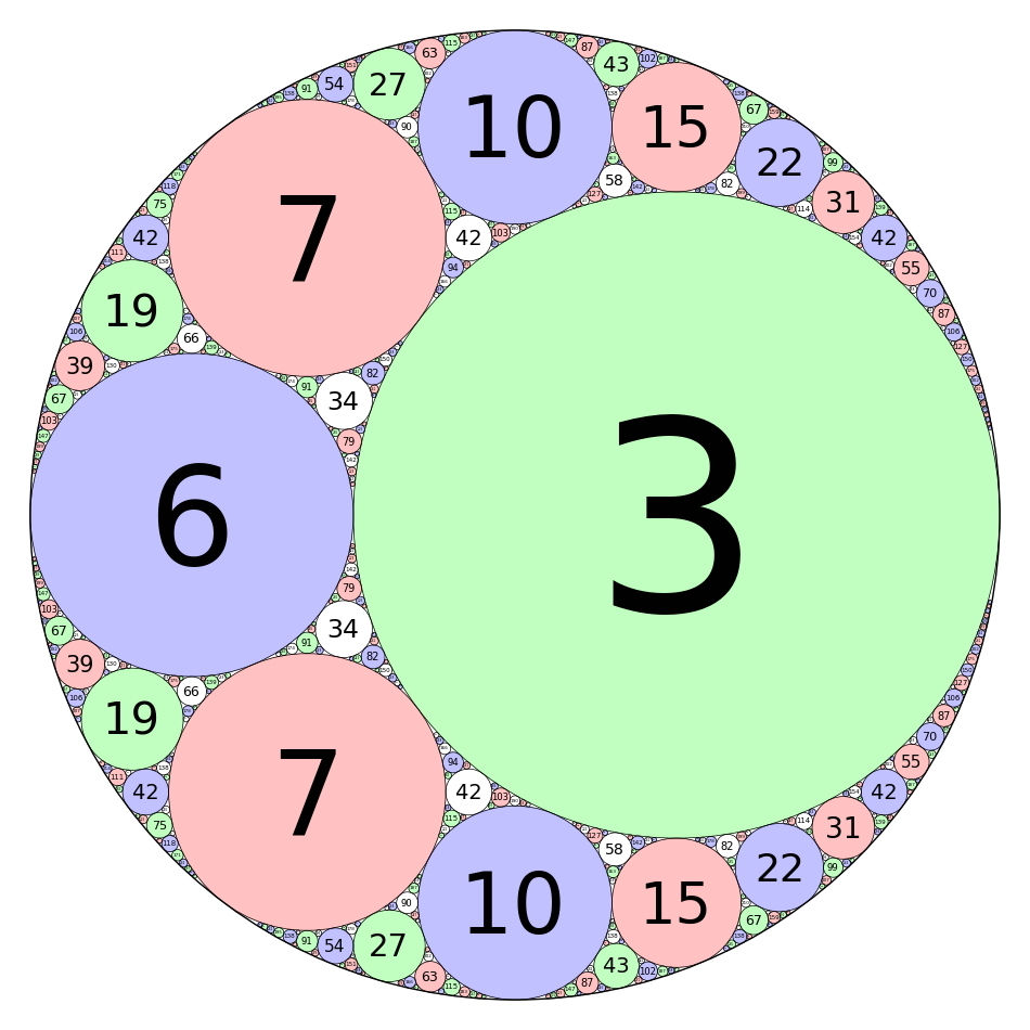
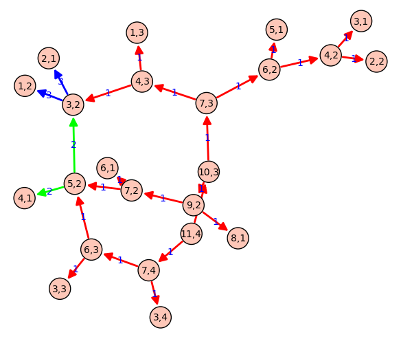
Call graph of a recursive function
def grafo_llamadas(f):
    class G(object):
        def __init__(self, f):
            self.f=f
            self.stack = []
            self.g   = DiGraph()
        def __call__(self, *args):
            if self.stack:
                sargs = ','.join(str(a) for a in args)
                last  = ','.join(str(a) for a in self.stack[-1])
                if self.g.has_edge(last, sargs):
                    l = self.g.edge_label(last, sargs)
                    self.g.set_edge_label(last, sargs, l + 1)
                else:
                    self.g.add_edge(last, sargs, 1)
            else:
                self.g   = DiGraph()
            self.stack.append(args)
            v = self.f(*args)
            self.stack.pop()
            return v
        def grafo(self):
            return self.g
    return G(f)

@grafo_llamadas
def particiones(n, k):
    if k == n:
        return [[1]*n]
    if k == 1:
        return [[n]]
    if not(0 < k < n):
        return []
    ls1 = [p+[1] for p in particiones(n-1, k-1)]
    ls2 = [[parte+1 for parte in p] for p in particiones(n-k, k)]
    return ls1 + ls2

particiones(13,5)
g = particiones.grafo()
g.show(edge_labels=True, figsize=(6,6), vertex_size=500, color_by_label=True)
{{{#D3js interactive version (just a screenshot here) edge_partition = [
- [edge for edge in g.edges() if edge[-1]==el] for el in set(g.edge_labels()) ]
g.show(method='js',
- edge_labels=True, vertex_labels=True, link_distance=90, charge=-400, link_strength=2, force_spring_layout=True, edge_partition=edge_partition)
}}}
