|
Size: 20262
Comment:
|
Size: 13560
Comment: switch from attachments to embedded images
|
| Deletions are marked like this. | Additions are marked like this. |
| Line 1: | Line 1: |
| == Pictures drawn by Sage == These pictures and images were drawn by [[http://www.sagemath.org|Sage]]. <<TableOfContents>> === Everywhere continuous, nowhere differentiable function === |
|
| Line 2: | Line 9: |
| {{{p = Graphics() | {{{#!python numbers=none p = Graphics() |
| Line 10: | Line 18: |
| [http://sage.math.washington.edu/home/wdj/art/cool-sage-pic-small1.png cool pic 1] * Math art by Tom Boothby: {{{ |
{{http://sage.math.washington.edu/home/wdj/art/cool-sage-pic-small1.png|cool pic 1}} === Mirrored balls in tachyon === {{{#!python numbers=none t = Tachyon(camera_center=(8.5,5,5.5), look_at=(2,0,0), raydepth=6, xres=1500, yres=1500) t.light((10,3,4), 1, (1,1,1)) t.texture('mirror', ambient=0.05, diffuse=0.05, specular=.9, opacity=0.9, color=(.8,.8,.8)) t.texture('grey', color=(.8,.8,.8), texfunc=7) ## try other values of texfunc too! t.plane((0,0,0),(0,0,1),'grey') t.sphere((4,-1,1), 1, 'mirror') t.sphere((0,-1,1), 1, 'mirror') t.sphere((2,-1,1), 0.5, 'mirror') t.sphere((2,1,1), 0.5, 'mirror') show(t) }}} {{http://sage.math.washington.edu/home/wdj/art/balls-mirrored-sage-tachyon1a.png|cool ray tracing pic}} === Math art by Tom Boothby === {{{#!python numbers=none |
| Line 37: | Line 63: |
| [http://sage.math.washington.edu/home/wdj/art/boothby-tachyon1.png cool pic 2] * Twisted cubic in tachyon: {{{ |
{{http://sage.math.washington.edu/home/wdj/art/boothby-tachyon1.png|cool pic 2}} === Twisted cubic in tachyon === {{{#!python numbers=none |
| Line 54: | Line 80: |
| [http://sage.math.washington.edu/home/wdj/art/boothby-tachyon2.png cool pic 3] * Reflections from four spheres in tachyon {{{ |
{{http://sage.math.washington.edu/home/wdj/art/boothby-tachyon2.png|cool pic 3}} === Reflections from four spheres in tachyon === {{{#!python numbers=none |
| Line 71: | Line 97: |
| [attachment:fourspheres.png] * A cone inside a sphere: {{{ |
{{attachment:fourspheres.png}} === A cone inside a sphere === {{{#!python numbers=none |
| Line 81: | Line 107: |
| http://sage.math.washington.edu/home/wdj/art/cone-inside-sphere.jpg * A cylinder inside a cone: {{{ |
{{http://sage.math.washington.edu/home/wdj/art/cone-inside-sphere.jpg}} === A cylinder inside a cone === {{{#!python numbers=none |
| Line 91: | Line 117: |
| http://sage.math.washington.edu/home/wdj/art/cylinder-inside-cone.jpg * An animation by Dean Moore: |
{{http://sage.math.washington.edu/home/wdj/art/cylinder-inside-cone.jpg}} === A hypotrochoid animation by Dean Moore === |
| Line 96: | Line 122: |
| http://sage.math.washington.edu/home/wdj/art/hypotrochoid_R_equals_7,_r_equals_2,_d=3.gif Inspiration: But a SAGE newbie & out to do projects & learn more, one day I was surfing Wikipedia and hit < http://en.wikipedia.org/wiki/Hypotrochoid >, saw the animated graph, and thought, ... "I bet I can make SAGE do that." Never one to back from a challenge, I did it. A few mistakes & wrong turns, at times some strong language & threatening the computer with violence, a few questions to SAGE support groups, but, I finally pounded out code that worked. I named it "Hypotrochoid," as animating this was the original inspiration, but the code easily animates other graphs. What this program does: This program animates (not just "draws," but "animates") graphs of several relations, the hypotrochoid, the hypocycloid, the limacon (or "limacon of Pascal"; SAGE doesn't like the French character in the original), the cardioid, the epitrochoid, and the epicycloid. The parametric equations that define a hypotrochoid follow; the parameter is *t*; for hypotrochoid we have R, r, d > 0, R > r > 0: {{{ x-coordinate: x = (R - r)*cos(t) + d*cos(((R - r)/r)*t) y-coordinate: y = (R - r)*sin(t) - d*sin(((R - r)/r)*t) }}} For a epitrochoid, the equations are: {{{ x = (R + r)*cos(t) - d*cos(((R + r)/r)*t) y = (R + r)*sin(t) - d*sin(((R + r)/r)*t) }}} The parametric equations are important in computing the period of the relation (below). These parametric equations live all over the Internet; Wikipedia has: ** for the hypochotroid: < http://en.wikipedia.org/wiki/Hypotrochoid >. See also < http://linuxgazette.net/133/luana.html > ** For the epitrochoid, see < http://en.wikipedia.org/wiki/Epitrochoid >. ** For the Limacon (SAGE completely choked and spewed error messages on the French character in the original, even in a comment) of Pascal, see < http://en.wikipedia.org/wiki/Lima%C3%A7on >. ** For the cardioid, see < http://en.wikipedia.org/wiki/Cardioid >. ** For the epitrochoid, see < < http://en.wikipedia.org/wiki/Epitrochoid > ** For the hypocycloid, see < http://en.wikipedia.org/wiki/Hypocycloid > ** For the Deltoid Curve, see < http://en.wikipedia.org/wiki/Deltoid_curve >. A few further comments: Some curves of the "roulette" family (see < http://en.wikipedia.org/wiki/Roulette_%28curve%29 > may be easily animated with this program, as follows: 1) The epitrochoid (use the negative of "small" radius *r*, easy, puts rotating circle on the outside. 2) The hypocycloid, by setting 0 < r < R, d = r. 3) The limacon (or "limacon of Pascal"; SAGE doesn't like the French character in the original), use r < 0, R = abs(r). 4) The epicycloid, use r < 0 (put rotating circle on outside), d = r 5) The cardioid, r < 0 d = r To draw different graphs, vary that parameters *R* (fixed circle's radius), *r* (rotating circle's radius), and *d* (length of "bar" from rotating circle), below; other parameters may be tweaked at will. Of some note, the *epitrochoid* is the "epicycle" curve of Ptolemaic system astronomy; one project is to animate some of the Ptolemaic system, but this is for the future. Program commences: {{{ #***************************************************************************** # Copyright (C) 2007 Dean Moore < [email protected] > # # Distributed under the terms of the GNU General Public License (GPL) # http://www.gnu.org/licenses/ #***************************************************************************** # Parameters that define the image: R = 5 # Fixed circle's radius. r = 3 # Rotating circle's radius, rotates about fixed circle's radius; make # this negative to place rotating circle on outside. d = 5 # Length of the "bar" extending from the center of the rotating circle. step = 0.025 # Size of "step" in below loops; the smaller the step, the more # "frames" in the final "movie" & the better the image, but the # slower the program runs -- and the more bytes to the image. figuresize = 4 # A constant, regulates size of final picture delayBetweenImages = 0 # A constant, delay between images in final "movie." colorOfFixedCircle = (0, 0, 1) # Colors of final image, colorOfRotatingCircle = (0, 1, 0) # all described by colorOfCenterPoint = (0, 0, 0) # names. colorOfBar = (0, 0, 0) colorOfCurve = (1, 0, 0) thicknessOfFixedCircle = 1 # Thickness of "fixed" circle that never moves. thicknessOfRotatingCircle = 1 # Thickness of circle that rotates. thicknessOfCenterOfRotatingCircle = 15 # Size of small circle's center. thicknessOfBar = 1 # Thickness of "bar" from rotating circle. penSize = 10 # Size of "pen" at end of the "bar." thicknessOfCurve = 0.5 # Thickness of final curve, really a lot of line segments. # End of parameters user can realistically vary. origin = (0, 0) # Maybe irrelevant, but NO MAGIC NUMBERS!! See # < http://en.wikipedia.org/wiki/Magic_number_(programming) >. # Comes from my days as a C/C++ programmer. # Graphic parameters, defined here: L = Graphics() # Graphics for the curve -- really a lot of segments of straight # lines. If the image looks choppy, drop variable *step* above. v = [] # Holds the curve from *L*, later converted to variable *curve*. # More parameters, all of which are defined by earlier parameters: rDiff = (R-r) # The rotating circle may exceed fixed circle; # values may be negative, so we may have a # negative value. We use this so much, we give # it a name. sizeOfGraph = max(R, abs(r) + abs(d), abs(R) - (r) + abs(d)) # Big as it can get -- may be # a liberal estimate. circle2PI = (abs(rDiff)/r).denom() # Number of rotations about 2*pi. It # takes a bit of thought, but see the above # parametric equations. An example is best: # picture R=8, r=6. We have # (rDiff)/r = (8-6)/6 = 2/6 = 1/3, reduced. For # the argument *((rDiff)/r)t* to get back to 2*pi # (i.e., zero) in cos(((R - r)/r)t) & sin(((R - r)/r)t), # we need to go 2*(3*pi). A pen & paper & some # scribbling makes this easy, be it this not # clear. The *abs* is probably irrelevant. limit = ceil(2*circle2PI/step) # Loop about circle this many times, by *step*. # Parameter *circle2PI* never is again used. Factor # of 2 is unavoidable, circle 2*pi; see below loops. }}} First: I use the same trig functions, over an over again. Why re-invent the wheel & waste computer time? Put the needed trig functions in arrays & "recycle" them as needed. {{{ sin1 = [ 0 for i in range(limit) ] # First sin2 = [ 0 for i in range(limit) ] # define cos1 = [ 0 for i in range(limit) ] # arrays, ... cos2 = [ 0 for i in range(limit) ] increment = 0 # Adding a bunch of numbers is more efficient than multiplying # *i*pi*step, but it is a trivial difference. multiplier = pi*rDiff/r # Efficiency! Don't repeat the same math # countless times. for i in srange(limit): # Note above definition of parameter *limit*, the # factor of 2, and the below trig functions. All # this program's loops go *limit*. sin1[i] = sin(increment*pi) # Now fill cos1[i] = cos(increment*pi) # arrays sin2[i] = sin(increment*multiplier) # with our trig cos2[i] = cos(increment*multiplier) # functions. increment += step # End *i*-loop. }}} The next are described by names, but a few notes: ** The parameter *fixedCircle* is merely a circle of radius *R* centered at the origin. I animated it, as that makes it appear in all frames. It never moves. ** The parameter *rotatingCircle* is more computation-intense. It's center is on the circle at *rDiff* from the edge of the fixed circle; its radius is *r*, and it rotates about the fixed circle a total of *circle2PI* times. Find any internet reference on these curves to see it. ** The parameter *centerPoints* is solely to make the rotating circle look nicer, a clear center. ** The parameter *bar* is the "bar" extending from the center of the rotating circle, that follows its rotation around the fixed circle. It always emanates from the same center as *fixedCircle*, -- see *fixedCircle* documentation, above -- and its terminal point comes from the parametric equation of a hypotrochoid (top). ** The parameter *pointAtPen* makes a point where the end of the bar draws the figure, of the same color as the final curve. Note it is at the same point as the terminal point of the "bar." {{{ fixedCircle = animate([circle(origin, R, # Centered at origin, radius *R*. rgbcolor=colorOfFixedCircle, thickness = thicknessOfFixedCircle) for i in srange(limit) # Animating loop. ], xmin=-sizeOfGraph, ymin=-sizeOfGraph, xmax= sizeOfGraph, ymax= sizeOfGraph, figsize=[figuresize, figuresize]) rotatingCircle = animate([circle((rDiff*cos1[i],rDiff*sin1[i]), r, # Note center, radius *r* thickness = thicknessOfRotatingCircle, rgbcolor=colorOfRotatingCircle) for i in srange(limit) # Animating loop ], xmin=-sizeOfGraph, ymin=-sizeOfGraph, xmax= sizeOfGraph, ymax= sizeOfGraph, figsize=[figuresize,figuresize]) centerPoints = animate([point((rDiff*cos1[i],rDiff*sin1[i]), # Center of *fixedCircle*. rgbcolor=colorOfCenterPoint, pointsize=thicknessOfCenterOfRotatingCircle) for i in srange(limit) # Animating loop ], xmin=-sizeOfGraph, ymin=-sizeOfGraph, xmax= sizeOfGraph, ymax= sizeOfGraph, figsize=[figuresize,figuresize]) bar = animate(line([(rDiff*cos1[i], rDiff*sin1[i]), # Starts here, and ... (d*cos2[i] + rDiff*cos1[i], # Ends at rDiff*sin1[i] - d*sin2[i]) # this point. ], thickness = thicknessOfBar, rgbcolor=colorOfBar) for i in srange(limit)) # Animating loop pointAtPen = animate([point((d*cos2[i]+rDiff*cos1[i], # End of pen, same x & y (rDiff)*sin1[i] - d*sin2[i]), # coordinates as endpoints of *bar* rgbcolor=colorOfCurve, pointsize=penSize) for i in srange(limit) # Animating loop ], xmin=-sizeOfGraph, ymin=-sizeOfGraph, xmax= sizeOfGraph, ymax= sizeOfGraph, figsize=[figuresize,figuresize]) # Prepare to draw the curve; we use four "important" variables: x0, x1, y0 & y1; # the line segment goes from (x0, y0) to (x1, y1): x0 = rDiff + d # Initial values of these variables; bumped up at bottom # of next loop -- see a graph or look at parametric equations # at zero to understand why it has this value. y0 = 0 # The "pen" out the small circle starts at this (x0, y0). # Now to compute the curve, in the next loop. Starts at zero, even if # this seems to make the first a junk computation; otherwise the output # looks weird: for i in srange(limit): # Parameter *circle2PI* is number of times we rotate # the "fixed" circle; limit=2*circle2PI; see above # documentation. x1 = rDiff*cos1[i] + d*cos2[i] # Initial, starting point of # the line; see parametric # equations. y1 = rDiff*sin1[i] - d*sin2[i] # Again, see the parametric # equation at top. # Now make the line: L += line([(x0, y0),(x1, y1)], rgbcolor = colorOfCurve , thickness=thicknessOfCurve) L.xmin(-sizeOfGraph) # Some nonsense L.ymin(-sizeOfGraph) # that needs done. L.xmax( sizeOfGraph) L.ymax( sizeOfGraph) x0 = x1 # Bump up these variables, start of y0 = y1 # next line segment is end of last. v.append(L) # *** End of loop *** # Stash curve *L* in the variable *v*. curve = animate(v) # Animate the curve, and ... # Show the entire "movie": (fixedCircle + rotatingCircle + pointAtPen + bar + centerPoints + curve).show(delay=delayBetweenImages) }}} We've shown the final image; done with program. |
This animation was moved to the section on the animate command : [[http://wiki.sagemath.org/animate#AhypotrochoidanimationbyDeanMoore]] === A simpler hypotrochoid === This animation was moved to the section on the animate command : [[http://wiki.sagemath.org/animate#Asimplerhypotrochoid]] === The witch of Maria Agnesi === by Marshall Hampton This animation was moved to the section on the animate command : [[http://wiki.sagemath.org/animate#ThewitchofMariaAgnesi]] === p-adic Seasons Greetings === |
| Line 405: | Line 137: |
| http://sage.math.washington.edu/home/wdj/art/padic-seasons-greetings.png | {{http://sage.math.washington.edu/home/wdj/art/padic-seasons-greetings.png}} |
| Line 409: | Line 141: |
| {{{ | {{{#!python numbers=none |
| Line 416: | Line 148: |
=== Lorentz butterfly === {{{#!python numbers=off """ Draws Loretz butterfly using matplotlib (2d) or jmol (3d). Written by Matthew Miller and William Stein. """ def butterfly2d(): """" EXAMPLE: sage: butterfly2d() """ g = Graphics() x1, y1 = 0, 0 from math import sin, cos, exp, pi for theta in srange( 0, 10*pi, 0.01 ): r = exp(cos(theta)) - 2*cos(4*theta) + sin(theta/12)^5 x = r * cos(theta) # Convert polar to rectangular coordinates y = r * sin(theta) xx = x*6 + 25 # Scale factors to enlarge and center the curve. yy = y*6 + 25 if theta != 0: l = line( [(x1, y1), (xx, yy)], rgbcolor=hue(theta/7 + 4) ) g = g + l x1, y1 = xx, yy g.show(dpi=100, axes=False) def butterfly3d(): """" EXAMPLE: sage: butterfly3d() """ g = point3d((0,0,0)) x1, y1 = 0, 0 from math import sin, cos, exp, pi for theta in srange( 0, 10*pi, 0.05): r = exp(cos(theta)) - 2*cos(4*theta) + sin(theta/12)^5 x = r * cos(theta) # Convert polar to rectangular coordinates y = r * sin(theta) xx = x*6 + 25 # Scale factors to enlarge and center the curve. yy = y*6 + 25 if theta != 0: l = line3d( [(x1, y1, theta), (xx, yy, theta)], rgbcolor=hue(theta/7 + 4) ) g = g + l x1, y1 = xx, yy g.show(dpi=100, axes=False) }}} {{http://sage.math.washington.edu/home/wdj/art/butterfly2d.png}} {{http://sage.math.washington.edu/home/wdj/art/butterfly3d.png}} === Feigenbaum diagram === Author: Pablo Angulo Posted to sage-devel 2008-09-13. See also https://sage.math.washington.edu:8101/home/pub/3 #Note: Mandelbrot set moved to interact/fractals {{{#!python numbers=off #Plots Feigenbaum diagram: divides the parameter interval [2,4] for mu #into N steps. For each value of the parameter, iterate the discrete #dynamical system x->mu*x*(1-x), drop the first M1 points in the orbit #and plot the next M2 points in a (mu,x) diagram N=200 M1=200 M2=200 x0=0.509434 puntos=[] for t in range(N): mu=2.0+2.0*t/N x=x0 for i in range(M1): x=mu*x*(1-x) for i in range(M2): x=mu*x*(1-x) puntos.append((mu,x)) point(puntos,pointsize=1) }}} {{attachment:feigenbaum.png}} === Sierpinski triangle === * This was a black+white Sierpinski triangle coded by Marshall Hampton, with some slight tweeking by David Joyner to add colors: {{{#!python numbers=none def sierpinski_seasons_greetings(): """ Code by Marshall Hampton. Colors by David Joyner. General depth by Rob Beezer. Copyright Marshall Hampton 2008, licensed creative commons, attribution share-alike. """ depth = 7 nsq = RR(3^(1/2))/2.0 tlist_old = [[[-1/2.0,0.0],[1/2.0,0.0],[0.0,nsq]]] tlist_new = tlist_old[:] for ind in range(depth): for tri in tlist_old: for p in tri: new_tri = [[(p[0]+x[0])/2.0, (p[1]+x[1])/2.0] for x in tri] tlist_new.append(new_tri) tlist_old = tlist_new[:] T = tlist_old N = 4^depth N1 = N - 3^depth q1 = sum([line(T[i]+[T[i][0]], rgbcolor = (0,1,0)) for i in range(N1)]) q2 = sum([line(T[i]+[T[i][0]], rgbcolor = (1,0,0)) for i in range(N1,N)]) show(q2+q1, figsize = [6,6*nsq], axes = False) }}} GIMP was used to add a Season's greetings message: {{http://sage.math.washington.edu/home/wdj/art/sierpinski-seasons-greetings-from-sage.png}} Also (thanks to Rob Beezer) available in poster form in pdf format: http://sage.math.washington.edu/home/wdj/art/seasons-greetings-sage.pdf, and in A4 size: http://sage.math.washington.edu/home/wdj/art/seasons-greetings-sage-a4.pdf. === The Tamer and the Lion by Provencal and Labbe === This animation was moved to the section on the animate command : [[http://wiki.sagemath.org/animate#TheTamerandtheLionbyProvencalandLabbe]] === Integral Curvature Apollonian Circle Packing === by Marshall Hampton and Carl Witty {{{ def kfun(k1,k2,k3,k4): """ The Descartes formula for the curvature of an inverted tangent circle. """ return 2*k1+2*k2+2*k3-k4 colorlist = [(1,0,1),(0,1,0),(0,0,1),(1,0,0)] def circfun(c1,c2,c3,c4): """ Computes the inversion of circle 4 in the first three circles. """ newk = kfun(c1[3],c2[3],c3[3],c4[3]) newx = (2*c1[0]*c1[3]+2*c2[0]*c2[3]+2*c3[0]*c3[3]-c4[0]*c4[3])/newk newy = (2*c1[1]*c1[3]+2*c2[1]*c2[3]+2*c3[1]*c3[3]-c4[1]*c4[3])/newk newcolor = c4[4] if newk > 0: newr = 1/newk elif newk < 0: newr = -1/newk else: newr = Infinity return [newx, newy, newr, newk, newcolor] def mcircle(circdata, label = False, thick = 1/10, cutoff = 2000, color = ''): """ Draws a circle from the data. label = True """ if color == '': color = colorlist[circdata[4]] if label==True and circdata[3] > 0 and circdata[2] > 1/cutoff: lab = text(str(circdata[3]),(circdata[0],circdata[1]), fontsize = \ 500*(circdata[2])^(.95), vertical_alignment = 'center', horizontal_alignment \ = 'center', rgbcolor = (0,0,0),zorder=10) else: lab = Graphics() circ = circle((circdata[0],circdata[1]), circdata[2], rgbcolor = (0,0,0), \ thickness = thick) circ = circ + circle((circdata[0],circdata[1]), circdata[2], rgbcolor = color, \ thickness = thick, fill=True, alpha = .4, zorder=0) return lab+circ def add_circs(c1, c2, c3, c4, cutoff = 300): """ Find the inversion of c4 through c1,c2,c3. Add the result to circlist, then (if the result is big enough) recurse. """ newcirc = circfun(c1, c2, c3, c4) if newcirc[3] < cutoff: circlist.append(newcirc) add_circs(newcirc, c1, c2, c3, cutoff = cutoff) add_circs(newcirc, c2, c3, c1, cutoff = cutoff) add_circs(newcirc, c3, c1, c2, cutoff = cutoff) zst1 = [0,0,1/2,-2,0] zst2 = [1/6,0,1/3,3,1] zst3 = [-1/3,0,1/6,6,2] zst4 = [-3/14,2/7,1/7,7,3] circlist = [zst1,zst2,zst3,zst4] add_circs(zst1,zst2,zst3,zst4,cutoff = 500) add_circs(zst2,zst3,zst4,zst1,cutoff = 500) add_circs(zst3,zst4,zst1,zst2,cutoff = 500) add_circs(zst4,zst1,zst2,zst3,cutoff = 500) circs = sum([mcircle(q, label = True, thick = 1/2) for q in \ circlist[1:]]) circs = circs + mcircle(circlist[0],color=(1,1,1),thick=1) circs.save('./Apollonian3.png',axes = False, figsize = [12,12], xmin = \ -1/2, xmax = 1/2, ymin = -1/2, ymax = 1/2) }}} {{attachment:Apollonian.png}} === Call graph of a recursive function === {{{ def grafo_llamadas(f): class G(object): def __init__(self, f): self.f=f self.stack = [] self.g = DiGraph() def __call__(self, *args): if self.stack: sargs = ','.join(str(a) for a in args) last = ','.join(str(a) for a in self.stack[-1]) if self.g.has_edge(last, sargs): l = self.g.edge_label(last, sargs) self.g.set_edge_label(last, sargs, l + 1) else: self.g.add_edge(last, sargs, 1) else: self.g = DiGraph() self.stack.append(args) v = self.f(*args) self.stack.pop() return v def grafo(self): return self.g return G(f) @grafo_llamadas def particiones(n, k): if k == n: return [[1]*n] if k == 1: return [[n]] if not(0 < k < n): return [] ls1 = [p+[1] for p in particiones(n-1, k-1)] ls2 = [[parte+1 for parte in p] for p in particiones(n-k, k)] return ls1 + ls2 particiones(13,5) g = particiones.grafo() g.show(edge_labels=True, figsize=(6,6), vertex_size=500, color_by_label=True) }}} {{attachment:call_graph_partitions_js_2.png}} {{attachment:call_graph_partitions.png}} |
Pictures drawn by Sage
These pictures and images were drawn by Sage.
Contents
-
Pictures drawn by Sage
- Everywhere continuous, nowhere differentiable function
- Mirrored balls in tachyon
- Math art by Tom Boothby
- Twisted cubic in tachyon
- Reflections from four spheres in tachyon
- A cone inside a sphere
- A cylinder inside a cone
- A hypotrochoid animation by Dean Moore
- A simpler hypotrochoid
- The witch of Maria Agnesi
- p-adic Seasons Greetings
- Lorentz butterfly
- Feigenbaum diagram
- Sierpinski triangle
- The Tamer and the Lion by Provencal and Labbe
- Integral Curvature Apollonian Circle Packing
- Call graph of a recursive function
Everywhere continuous, nowhere differentiable function
- Everywhere continuous, nowhere differentiable function (in the infinite limit, anyway):
p = Graphics()
for n in range(1,20):
  f = lambda x: sum([sin(x*3^i)/(2^i) for i in range(1,n)])
  p += plot(f,0,float(pi/3),plot_points=2000,rgbcolor=hue(n/20))

p.show(xmin=0, ymin=0,dpi=250)

Mirrored balls in tachyon
t = Tachyon(camera_center=(8.5,5,5.5), look_at=(2,0,0), raydepth=6, xres=1500, yres=1500)
t.light((10,3,4), 1, (1,1,1))
t.texture('mirror', ambient=0.05, diffuse=0.05, specular=.9, opacity=0.9, color=(.8,.8,.8))
t.texture('grey', color=(.8,.8,.8), texfunc=7) ## try other values of texfunc too!
t.plane((0,0,0),(0,0,1),'grey')
t.sphere((4,-1,1), 1, 'mirror')
t.sphere((0,-1,1), 1, 'mirror')
t.sphere((2,-1,1), 0.5, 'mirror')
t.sphere((2,1,1), 0.5, 'mirror')
show(t)

Math art by Tom Boothby
# Author: Tom Boothby
# This is a remake of an old art piece I made in POVRay


t = Tachyon(xres=1000,yres=600, camera_center=(1,0,5), antialiasing=3)
t.light((4,3,2), 0.2, (1,1,1))
t.texture('t0', ambient=0.1, diffuse=0.9, specular=0.5, opacity=1.0, color=(1.0,1,1))
t.texture('t1', ambient=0.5, diffuse=0.5, specular=0.0, opacity=1.0, color=(0,0,0))
t.texture('t2', ambient=0.2, diffuse=0.7, specular=0, opacity=0.7, color=(.5,.5,.5))
t.texture('t3', ambient=.9, diffuse=5, specular=0,opacity=.1, color=(1,0,0))
t.sphere((1,0,0), 30, 't2')


k=0
for i in srange(-pi*10,0,.01):
  k += 1
  t.sphere((cos(i/10)-.1, sin(i/10)*cos(i), sin(i/10)*sin(i)), 0.1, 't0')
  t.sphere((cos(i/10) + 2.1, sin(i/10)*cos(i), sin(i/10)*sin(i)), 0.1, 't1')

t.show(verbose=1)

Twisted cubic in tachyon
t = Tachyon(xres=512,yres=512, camera_center=(5,0,0))
t.light((4,3,2), 0.2, (1,1,1))
t.texture('t0', ambient=0.1, diffuse=0.9, specular=0.5, opacity=1.0, color=(1.0,0,0))
t.texture('t1', ambient=0.1, diffuse=0.9, specular=0.3, opacity=1.0, color=(0,1.0,0))
t.texture('t2', ambient=0.2, diffuse=0.7, specular=0.5, opacity=0.7, color=(0,0,1.0))
k=0
for i in srange(-5,1.5,0.1):
    k += 1
    t.sphere((i,i^2-0.5,i^3), 0.1, 't%s'%(k%3))

t.show()

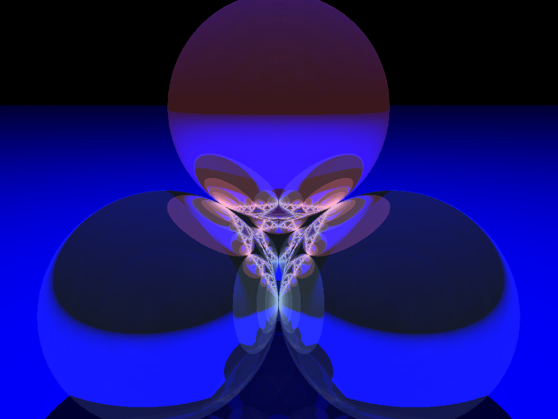
Reflections from four spheres in tachyon
t6 = Tachyon(camera_center=(0,-4,1), xres = 800, yres = 600, raydepth = 12, aspectratio=.75, antialiasing = True)
t6.light((0.02,0.012,0.001), 0.01, (1,0,0))
t6.light((0,0,10), 0.01, (0,0,1))
t6.texture('s', color = (.8,1,1), opacity = .9, specular = .95, diffuse = .3, ambient = 0.05)
t6.texture('p', color = (0,0,1), opacity = 1, specular = .2)
t6.sphere((-1,-.57735,-0.7071),1,'s')
t6.sphere((1,-.57735,-0.7071),1,'s')
t6.sphere((0,1.15465,-0.7071),1,'s')
t6.sphere((0,0,0.9259),1,'s')
t6.plane((0,0,-1.9259),(0,0,1),'p')
t6.show()
A cone inside a sphere
sage: u,v = var("u,v")
sage: p1 = parametric_plot3d([cos(u)*v, sin(u)*v, 3*v/2-1/3], (u, 0, 2*pi), (v, 0, 0.95),plot_points=[20,20])
sage: p2 = sphere((0,0,2/3), color='red', opacity=0.5, aspect_ratio=[1,1,1])
sage: show(p1+p2)

A cylinder inside a cone
sage: u,v = var("u,v")
sage: p1 = parametric_plot3d([cos(u)*v, sin(u)*v, 3/2-3*v/2], (u, 0, 2*pi), (v, 0, 1.5), opacity = 0.5, plot_points=[20,20])
sage: p2 = parametric_plot3d([cos(u)/2, sin(u)/2, v-3/4], (u, 0, 2*pi), (v, 0, 3/2), plot_points=[20,20])
sage: show(p1+p2)

A hypotrochoid animation by Dean Moore
Hypotrochoid. Written by Dean Moore, February 2008
This animation was moved to the section on the animate command : http://wiki.sagemath.org/animate#AhypotrochoidanimationbyDeanMoore
A simpler hypotrochoid
This animation was moved to the section on the animate command : http://wiki.sagemath.org/animate#Asimplerhypotrochoid
The witch of Maria Agnesi
by Marshall Hampton
This animation was moved to the section on the animate command : http://wiki.sagemath.org/animate#ThewitchofMariaAgnesi
p-adic Seasons Greetings
- I know this is early, but thanks to Robert Bradshaw's p-adic plot function, here is a p-adic Seasons Greetings:

This is the code:
sage: P1 = Zp(3).plot(rgbcolor=(0,1,0))
sage: P2 = Zp(7).plot(rgbcolor=(1,0,0))
sage: P3 = text("$Seasons$ $Greetings$ ",(0.0,1.8))
sage: P4 = text("$from$ $everyone$ $at$ sagemath.org!",(0.1,-1.6))
sage: (P1+P2+P3+P4).show(axes=False)
Lorentz butterfly
"""
Draws Loretz butterfly using matplotlib (2d) or jmol (3d).
Written by Matthew Miller and William Stein.

"""

def butterfly2d():
    """"
    EXAMPLE:
        sage: butterfly2d()
    """
    g = Graphics()
    x1, y1 = 0, 0
    from math import sin, cos, exp, pi
    for theta in srange( 0, 10*pi, 0.01 ):
        r = exp(cos(theta)) - 2*cos(4*theta) + sin(theta/12)^5
        x = r * cos(theta)  # Convert polar to rectangular coordinates
        y = r * sin(theta)
        xx = x*6 + 25       # Scale factors to enlarge and center the curve.
        yy = y*6 + 25
        if theta != 0:
            l = line( [(x1, y1), (xx, yy)], rgbcolor=hue(theta/7 + 4) )
            g = g + l
            x1, y1 = xx, yy
    g.show(dpi=100, axes=False)

def butterfly3d():
    """"
    EXAMPLE:
        sage: butterfly3d()
    """
    g = point3d((0,0,0))
    x1, y1 = 0, 0
    from math import sin, cos, exp, pi
    for theta in srange( 0, 10*pi, 0.05):
        r = exp(cos(theta)) - 2*cos(4*theta) + sin(theta/12)^5
        x = r * cos(theta)  # Convert polar to rectangular coordinates
        y = r * sin(theta)
        xx = x*6 + 25       # Scale factors to enlarge and center the curve.
        yy = y*6 + 25
        if theta != 0:
            l = line3d( [(x1, y1, theta), (xx, yy, theta)],
            rgbcolor=hue(theta/7 + 4) )
            g = g + l
            x1, y1 = xx, yy
    g.show(dpi=100, axes=False)


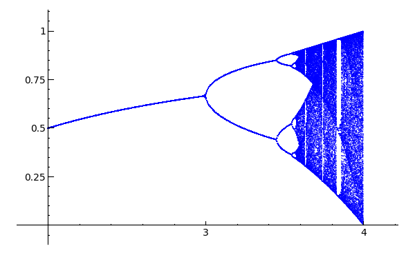
Feigenbaum diagram
Author: Pablo Angulo Posted to sage-devel 2008-09-13. See also https://sage.math.washington.edu:8101/home/pub/3 #Note: Mandelbrot set moved to interact/fractals
#Plots Feigenbaum diagram: divides the parameter interval [2,4] for mu
#into N steps. For each value of the parameter, iterate the discrete
#dynamical system x->mu*x*(1-x), drop the first M1 points in the orbit
#and plot the next M2 points in a (mu,x) diagram

N=200
M1=200
M2=200
x0=0.509434

puntos=[]
for t in range(N):
   mu=2.0+2.0*t/N
   x=x0
   for i in range(M1):
       x=mu*x*(1-x)
   for i in range(M2):
       x=mu*x*(1-x)
       puntos.append((mu,x))
point(puntos,pointsize=1)
Sierpinski triangle
- This was a black+white Sierpinski triangle coded by Marshall Hampton, with some slight tweeking by David Joyner to add colors:
def sierpinski_seasons_greetings():
    """
    Code by Marshall Hampton.
    Colors by David Joyner.
    General depth by Rob Beezer.
    Copyright Marshall Hampton 2008, licensed
    creative commons, attribution share-alike.
    """
    depth = 7
    nsq = RR(3^(1/2))/2.0
    tlist_old = [[[-1/2.0,0.0],[1/2.0,0.0],[0.0,nsq]]]
    tlist_new = tlist_old[:]
    for ind in range(depth):
       for tri in tlist_old:
           for p in tri:
               new_tri = [[(p[0]+x[0])/2.0, (p[1]+x[1])/2.0] for x in tri]
               tlist_new.append(new_tri)
       tlist_old = tlist_new[:]
    T = tlist_old
    N  = 4^depth
    N1 = N - 3^depth
    q1 = sum([line(T[i]+[T[i][0]], rgbcolor = (0,1,0)) for i in range(N1)])
    q2 = sum([line(T[i]+[T[i][0]], rgbcolor = (1,0,0)) for i in range(N1,N)])
    show(q2+q1, figsize = [6,6*nsq], axes = False)
GIMP was used to add a Season's greetings message:

Also (thanks to Rob Beezer) available in poster form in pdf format: http://sage.math.washington.edu/home/wdj/art/seasons-greetings-sage.pdf, and in A4 size: http://sage.math.washington.edu/home/wdj/art/seasons-greetings-sage-a4.pdf.
The Tamer and the Lion by Provencal and Labbe
This animation was moved to the section on the animate command : http://wiki.sagemath.org/animate#TheTamerandtheLionbyProvencalandLabbe
Integral Curvature Apollonian Circle Packing
by Marshall Hampton and Carl Witty
def kfun(k1,k2,k3,k4):
    """
    The Descartes formula for the curvature of an inverted tangent circle.
    """
    return 2*k1+2*k2+2*k3-k4


colorlist = [(1,0,1),(0,1,0),(0,0,1),(1,0,0)]

def circfun(c1,c2,c3,c4):
    """
    Computes the inversion of circle 4 in the first three circles.
    """
    newk = kfun(c1[3],c2[3],c3[3],c4[3])
    newx = (2*c1[0]*c1[3]+2*c2[0]*c2[3]+2*c3[0]*c3[3]-c4[0]*c4[3])/newk
    newy = (2*c1[1]*c1[3]+2*c2[1]*c2[3]+2*c3[1]*c3[3]-c4[1]*c4[3])/newk
    newcolor = c4[4]
    if newk > 0:
        newr = 1/newk
    elif newk < 0:
        newr = -1/newk
    else:
        newr = Infinity
    return [newx, newy, newr, newk, newcolor]

def mcircle(circdata, label = False, thick = 1/10, cutoff = 2000, color = ''):
    """
    Draws a circle from the data.  label = True
    """
    if color == '':
        color = colorlist[circdata[4]]
    if label==True and circdata[3] > 0 and circdata[2] > 1/cutoff:
        lab = text(str(circdata[3]),(circdata[0],circdata[1]), fontsize = \
500*(circdata[2])^(.95), vertical_alignment = 'center', horizontal_alignment \
= 'center', rgbcolor = (0,0,0),zorder=10)
    else:
        lab = Graphics()
    circ = circle((circdata[0],circdata[1]), circdata[2], rgbcolor = (0,0,0), \
thickness = thick)
    circ = circ + circle((circdata[0],circdata[1]), circdata[2], rgbcolor = color, \
thickness = thick, fill=True, alpha = .4, zorder=0)
    return lab+circ

def add_circs(c1, c2, c3, c4, cutoff = 300):
    """
    Find the inversion of c4 through c1,c2,c3.  Add the result to circlist,
    then (if the result is big enough) recurse.
    """
    newcirc = circfun(c1, c2, c3, c4)
    if newcirc[3] < cutoff:
        circlist.append(newcirc)
        add_circs(newcirc, c1, c2, c3, cutoff = cutoff)
        add_circs(newcirc, c2, c3, c1, cutoff = cutoff)
        add_circs(newcirc, c3, c1, c2, cutoff = cutoff)

zst1 = [0,0,1/2,-2,0]
zst2 = [1/6,0,1/3,3,1]
zst3 = [-1/3,0,1/6,6,2]
zst4 = [-3/14,2/7,1/7,7,3]

circlist = [zst1,zst2,zst3,zst4]
add_circs(zst1,zst2,zst3,zst4,cutoff = 500)
add_circs(zst2,zst3,zst4,zst1,cutoff = 500)
add_circs(zst3,zst4,zst1,zst2,cutoff = 500)
add_circs(zst4,zst1,zst2,zst3,cutoff = 500)

circs = sum([mcircle(q, label = True, thick = 1/2) for q in \
circlist[1:]])
circs = circs + mcircle(circlist[0],color=(1,1,1),thick=1)
circs.save('./Apollonian3.png',axes = False, figsize = [12,12], xmin = \
-1/2, xmax = 1/2, ymin = -1/2, ymax = 1/2)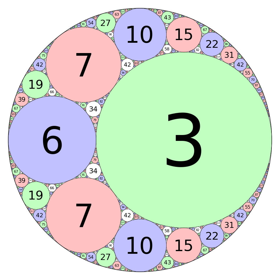
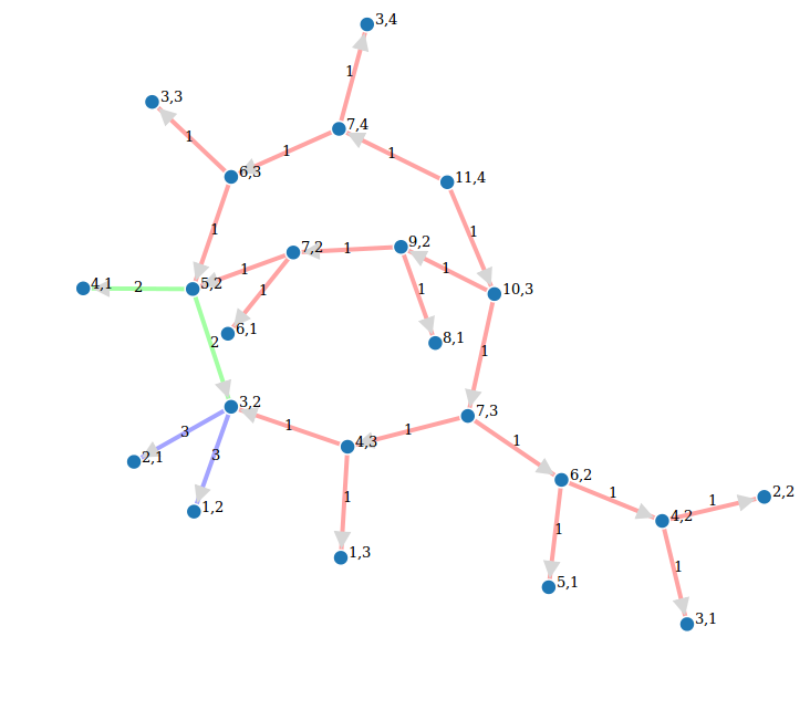
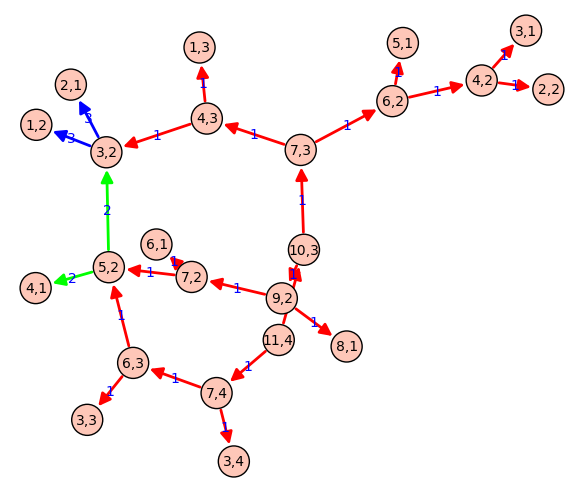
Call graph of a recursive function
def grafo_llamadas(f):
    class G(object):
        def __init__(self, f):
            self.f=f
            self.stack = []
            self.g   = DiGraph()
        def __call__(self, *args):
            if self.stack:
                sargs = ','.join(str(a) for a in args)
                last  = ','.join(str(a) for a in self.stack[-1])
                if self.g.has_edge(last, sargs):
                    l = self.g.edge_label(last, sargs)
                    self.g.set_edge_label(last, sargs, l + 1)
                else:
                    self.g.add_edge(last, sargs, 1)
            else:
                self.g   = DiGraph()
            self.stack.append(args)
            v = self.f(*args)
            self.stack.pop()
            return v
        def grafo(self):
            return self.g
    return G(f)

@grafo_llamadas
def particiones(n, k):
    if k == n:
        return [[1]*n]
    if k == 1:
        return [[n]]
    if not(0 < k < n):
        return []
    ls1 = [p+[1] for p in particiones(n-1, k-1)]
    ls2 = [[parte+1 for parte in p] for p in particiones(n-k, k)]
    return ls1 + ls2

particiones(13,5)
g = particiones.grafo()
g.show(edge_labels=True, figsize=(6,6), vertex_size=500, color_by_label=True)