|
Size: 9287
Comment:
|
Size: 10643
Comment:
|
| Deletions are marked like this. | Additions are marked like this. |
| Line 9: | Line 9: |
| {{{ | {{{#!sagecell |
| Line 132: | Line 132: |
| {{{ | {{{#!sagecell from scipy.optimize import leastsq |
| Line 135: | Line 136: |
| import time current_year = time.localtime().tm_year |
|
| Line 144: | Line 147: |
| trdf = RealField(16) @interact def mauna_loa_co2(start_date = slider(1958,2010,1,1958), end_date = slider(1958, 2010,1,2009)): |
npi = RDF(pi) @interact(layout=[['start_date'],['end_date'],['show_linear_fit','show_nonlinear_fit']]) def mauna_loa_co2(start_date = slider(1958,current_year,1,1958), end_date = slider(1958, current_year,1,current_year-1), show_linear_fit = checkbox(default=True), show_nonlinear_fit = checkbox(default=False)): |
| Line 149: | Line 152: |
| sel_data = [[q[2],q[4]] for q in datalines if start_date < q[2] < end_date] | html(htmls1+htmls2) sel_data = [[q[2],q[4]] for q in datalines if start_date <= q[2] <= end_date] outplot = list_plot(sel_data, plotjoined=True, rgbcolor=(1,0,0)) if show_nonlinear_fit: def powerlaw(t,a): return sel_data[0][1] + a[0]*(t-sel_data[0][0])^(a[1]) def res_fun(a): return [q[1]-powerlaw(q[0],a) for q in sel_data] def fitcos(t,a): return a[0]*cos(t*2*npi+a[1])+a[2]*cos(t*4*npi+a[3]) def res_fun2(a): return [q[1]-fitcos(q[0],a) for q in resids] a1 = leastsq(res_fun,[1/2.4,1.3])[0] resids = [[q[0],q[1] - powerlaw(q[0],a1)] for q in sel_data] a2 = leastsq(res_fun2, [3,0,1,0])[0] r2_plot = list_plot([[q[0],powerlaw(q[0],a1)+fitcos(q[0],a2)] for q in resids], rgbcolor='green',plotjoined=True) outplot = outplot + r2_plot var('t') formula1 = '%.2f+%.2f(t - %d)^%.2f'%(sel_data[0][1],a1[0],sel_data[0][0],a1[1]) formula2 = '%.2fcos(2 pi t + %.2f)+%.2f cos(4 pi t + %.2f)'%(a2[0],a2[1],a2[2],a2[3]) html('Nonlinear fit: <br>%s<br>'%(formula1+'+'+formula2)) if show_linear_fit: slope, intercept, r, ttprob, stderr = Stat.linregress(sel_data) outplot = outplot + plot(slope*x+intercept,start_date,end_date) html('Linear regression slope: %.2f ppm/year; correlation coefficient: %.2f'%(slope,r)) var('x,y') |
| Line 152: | Line 180: |
| slope, intercept, r, ttprob, stderr = Stat.linregress(sel_data) html(htmls1+htmls2+'<h4>Linear regression slope: ' + str(trdf(slope)) + ' ppm/year; correlation coefficient: ' + str(trdf(r)) + '</h4>') var('x,y') show(list_plot(sel_data, plotjoined=True, rgbcolor=(1,0,0)) + plot(slope*x+intercept,start_date,end_date), xmin = start_date, ymin = c_min-2, axes = True, xmax = end_date, ymax = c_max+3, frame = False) |
show(outplot, xmin = start_date, ymin = c_min-2, axes = True, xmax = end_date, ymax = c_max+3, frame = False) |
| Line 162: | Line 187: |
| {{{ | {{{#!sagecell |
| Line 202: | Line 227: |
| {{{ | {{{#!sagecell |
Sage Interactions - Web applications
goto interact main page
Contents
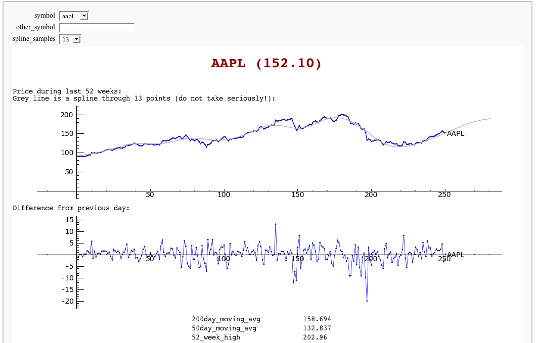
Stock Market data, fetched from Yahoo and Google
by William Stein

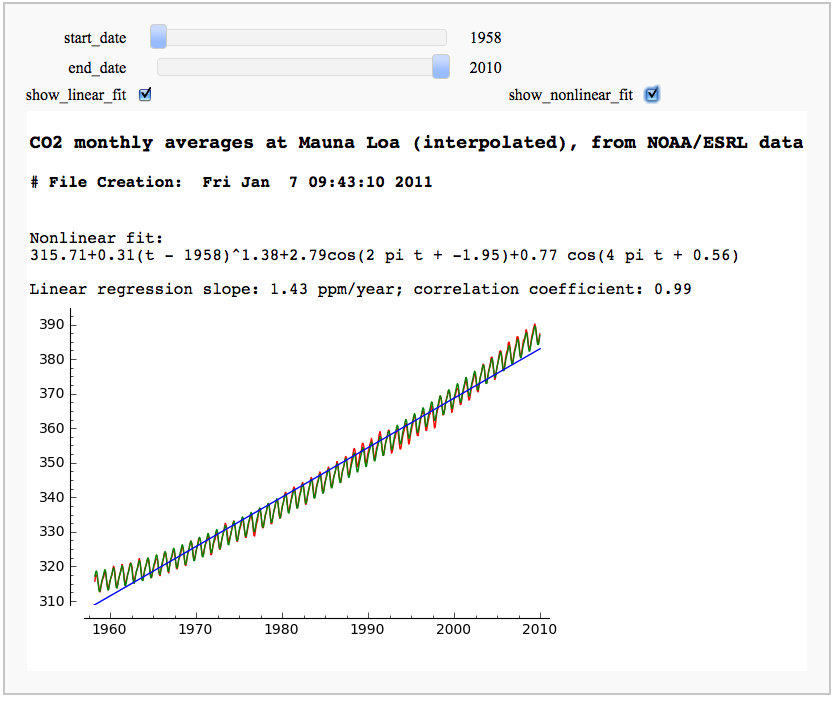
CO2 data plot, fetched from NOAA
by Marshall Hampton
While support for R is rapidly improving, scipy.stats has a lot of useful stuff too. This only scratches the surface.

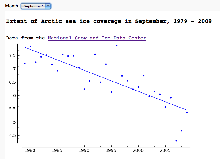
Arctic sea ice extent data plot, fetched from NSIDC
by Marshall Hampton

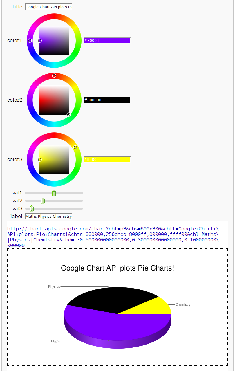
Pie Chart from the Google Chart API
by Harald Schilly

