|
Size: 7630
Comment:
|
Size: 14153
Comment:
|
| Deletions are marked like this. | Additions are marked like this. |
| Line 7: | Line 7: |
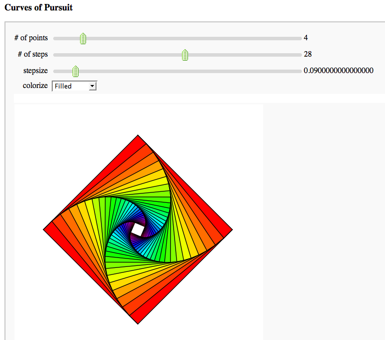
| == Curves of Pursuit == by Marshall Hampton. {{{#!sagecell npi = RDF(pi) from math import cos,sin def rot(t): return matrix([[cos(t),sin(t)],[-sin(t),cos(t)]]) def pursuit(n,x0,y0,lamb,steps = 100, threshold = .01): paths = [[[x0,y0]]] for i in range(1,n): rx,ry = list(rot(2*npi*i/n)*vector([x0,y0])) paths.append([[rx,ry]]) oldpath = [x[-1] for x in paths] for q in range(steps): diffs = [[oldpath[(j+1)%n][0]-oldpath[j][0],oldpath[(j+1)%n][1]-oldpath[j][1]] for j in range(n)] npath = [[oldpath[j][0]+lamb*diffs[j][0],oldpath[j][1]+lamb*diffs[j][1]] for j in range(n)] for j in range(n): paths[j].append(npath[j]) oldpath = npath return paths html('<h3>Curves of Pursuit</h3>') @interact def curves_of_pursuit(n = slider([2..20],default = 5, label="# of points"),steps = slider([floor(1.4^i) for i in range(2,18)],default = 10, label="# of steps"), stepsize = slider(srange(.01,1,.01),default = .2, label="stepsize"), colorize = selector(['BW','Line color', 'Filled'],default = 'BW')): outpaths = pursuit(n,0,1,stepsize, steps = steps) mcolor = (0,0,0) outer = line([q[0] for q in outpaths]+[outpaths[0][0]], rgbcolor = mcolor) polys = Graphics() if colorize=='Line color': colors = [hue(j/steps,1,1) for j in range(len(outpaths[0]))] elif colorize == 'BW': colors = [(0,0,0) for j in range(len(outpaths[0]))] else: colors = [hue(j/steps,1,1) for j in range(len(outpaths[0]))] polys = sum([polygon([outpaths[(i+1)%n][j+1],outpaths[(i+1)%n][j], outpaths[i][j+1]], rgbcolor = colors[j]) for i in range(n) for j in range(len(outpaths[0])-1)]) #polys = polys[0] colors = [(0,0,0) for j in range(len(outpaths[0]))] nested = sum([line([q[j] for q in outpaths]+[outpaths[0][j]], rgbcolor = colors[j]) for j in range(len(outpaths[0]))]) lpaths = [line(x, rgbcolor = mcolor) for x in outpaths] show(sum(lpaths)+nested+polys, axes = False, figsize = [5,5], xmin = -1, xmax = 1, ymin = -1, ymax =1) }}} {{attachment:pcurves.png}} |
|
| Line 8: | Line 51: |
| {{{ | {{{#!sagecell |
| Line 78: | Line 121: |
| {{{ | {{{#!sagecell |
| Line 91: | Line 134: |
| {{{ | {{{#!sagecell |
| Line 114: | Line 157: |
| {{{ | {{{#!sagecell |
| Line 120: | Line 163: |
| @interact def _(band_number = selector(range(1,5)), current_color = Color('red')): |
@interact def _(band_number = selector(range(1,5)), current_color = Color('red'), auto_update=False): |
| Line 131: | Line 175: |
| {{{ | {{{#!sagecell |
| Line 142: | Line 186: |
| == Interactive 2d Plotting == | == Interactive 2D Plotting == |
| Line 144: | Line 188: |
| {{{ | {{{#!sagecell |
| Line 174: | Line 218: |
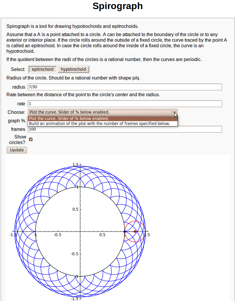
| {{attachment:interactive_2d_plotting.png}} == Interact with matplotlib == {{{#!sagecell # Simple example demonstrating how to interact with matplotlib directly. # Comment plt.clf() to get the plots overlay in each update. # Gokhan Sever & Harald Schilly (2010-01-24) from scipy import stats import numpy as np import matplotlib.pyplot as plt @interact def plot_norm(loc=(0,(0,10)), scale=(1,(1,10))): rv = stats.norm(loc, scale) x = np.linspace(-10,10,1000) plt.plot(x,rv.pdf(x)) plt.grid(True) plt.savefig('plt.png') plt.clf() }}} {{attachment:matplotlib_interact.png}} == Spirograph == {{{#!sagecell #---------------------------# # Javier Pérez Lázaro # # Logroño (Spain) # # [email protected] # #---------------------------# #introduction html('<h1><center>Spirograph</center></h1>') text1='Spirograph is a tool for drawing hypotrochoids and epitrochoids.' text2='Assume that a A is a point attached to a circle. A can be attached to the boundary of the circle or to any exterior or interior place. If the circle rolls around the outside of a fixed circle, the curve traced by the point A is called an epitrochoid. In case the circle rolls around the inside of a fixed circle, the curve is an hypotrochoid.' text3='If the quotient between the radii of the circles is a rational number, then the curves are periodic.' #the code @interact def fun( tex1=text_control(text1), tex2=text_control(text2), tex3=text_control(text3), h=('Select:',list(['epitrochoid','hypotrochoid'])), tex4=text_control('Radius of the circle. Should be a rational number with shape p/q.'), b=input_box(default=7/30,label='radius'), tex5=text_control("Rate between the distance of the point to the circle's center and the radius."), rate=input_box(default=1), u=selector(['Plot the curve. Slider of % below enabled.', 'Build an animation of the plot with the number of frames specified below.'],label='Choose:'), per=slider(0,100,1,default=100,label='graph %'), frames=100, cir_bool=checkbox(True, "Show circles?"), auto_update=false): draw=True if h=='hypotrochoid' and (b>=1 or b<=0): print "In a hypotrochoid, radius must be between 0 and 1." draw=False if h=='epitrochoid' and b<=0: print "In a epitrochoid, radius must be positive" draw=False if draw==True: if h=='hypotrochoid': b=-b var('t') cx=(1+b)*cos(t*b/(1+b)) cy=(1+b)*sin(t*b/(1+b)) px=cx-b*rate*cos(t) py=cy-b*rate*sin(t) axeM=1+max([0,b+abs(b)*rate]) if u=='Plot the curve. Slider of % below enabled.': tMax=pi*denominator(b/(b+1))*per/50 L=parametric_plot((px,py),(t,0,max([0.001,tMax])),plot_points=10*rate*tMax) if cir_bool: p=point((px(t=tMax),py(t=tMax)),pointsize=30,color='blue') c=point((cx(t=tMax),cy(t=tMax)),pointsize=30,color='red') cir=circle((cx(t=tMax),cy(t=tMax)),b,color='red') lin=line([(cx(t=tMax),cy(t=tMax)),(px(t=tMax),py(t=tMax))]) L+=circle((0,0),1)+cir+lin+p+c show(L,aspect_ratio=1,xmin=-axeM,xmax=axeM,ymin=-axeM,ymax=axeM) if u=='Build an animation of the plot with the number of frames specified below.': tMax=2*pi*denominator(b/(b+1)) step=tMax/(frames-1) curva=Graphics() v=[] for a in srange(step,tMax,step): curva+=parametric_plot((px,py),(t,a-step,a)) L=curva if cir_bool: cx_a=cx(t=a) cy_a=cy(t=a) px_a=cx_a-b*rate*cos(a) py_a=cy_a-b*rate*sin(a) p=point((px_a,py_a),pointsize=30,color='blue') c=point((cx_a,cy_a),pointsize=30,color='red') cir=circle((cx_a,cy_a),b,color='red') lin=line([(cx_a,cy_a),(px_a,py_a)]) L+=circle((0,0),1)+cir+lin+c+p v.append(L) animate(v,xmin=-axeM,xmax=axeM,ymin=-axeM,ymax=axeM,aspect_ratio=1).show() }}} {{attachment:interactive_animate_spirograph.png}} |
Sage Interactions - Graphics
goto interact main page
Contents
Curves of Pursuit
by Marshall Hampton.
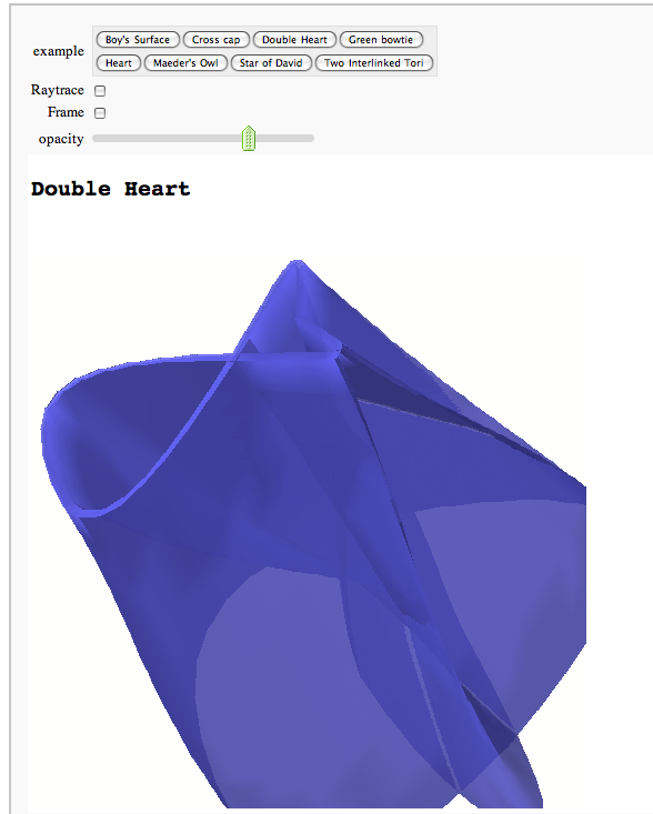
Catalog of 3D Parametric Plots
Interactive rotatable raytracing with Tachyon3d
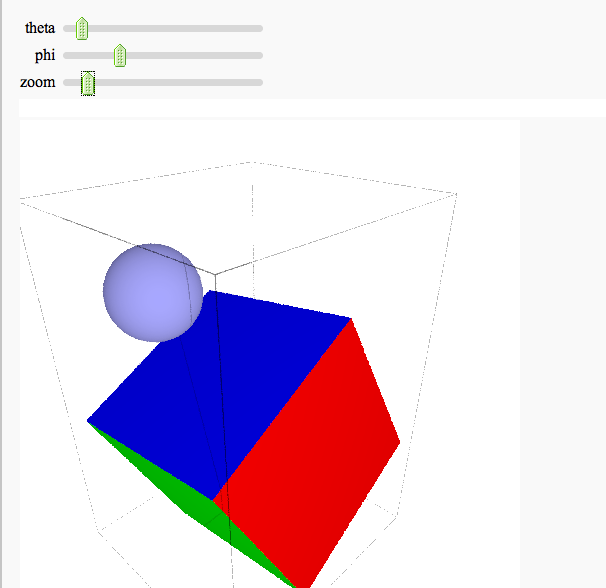
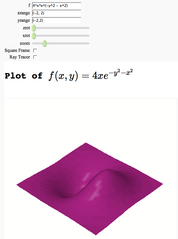
Interactive 3d plotting
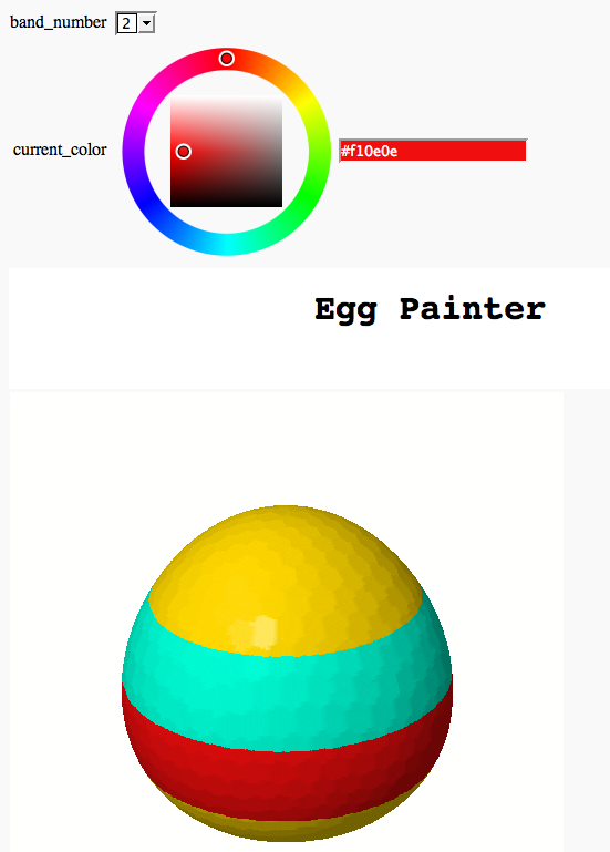
Somewhat Silly Egg Painter
by Marshall Hampton (refereed by William Stein)
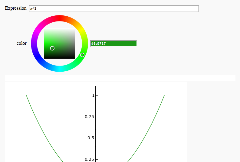
Plot Coloring
by Timothy Clemans
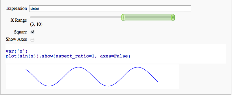
Interactive 2D Plotting
by Timothy Clemans
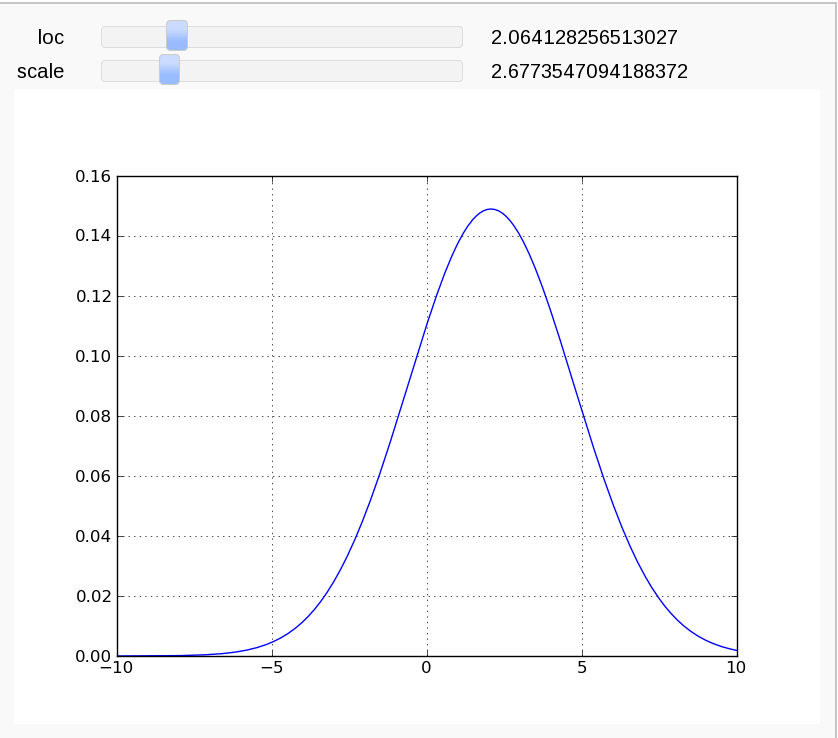
Interact with matplotlib
Spirograph
