|
Size: 62694
Comment:
|
Size: 63360
Comment:
|
| Deletions are marked like this. | Additions are marked like this. |
| Line 118: | Line 118: |
| html('<h2>Tangent line grapher</h2>') | pretty_print(html('<h2>Tangent line grapher</h2>')) |
| Line 158: | Line 158: |
| html('<h3>Numerical integrals with the midpoint rule</h3>') html('$\int_{a}^{b}{f(x) dx} {\\approx} \sum_i{f(x_i) \Delta x}$') |
pretty_print(html('<h3>Numerical integrals with the midpoint rule</h3>')) pretty_print(html('$\int_{a}^{b}{f(x) dx} {\\approx} \sum_i{f(x_i) \Delta x}$')) |
| Line 249: | Line 249: |
| html('$r=' + latex(b+sin(a1*t)^n1 + cos(a2*t)^n2)+'$') | pretty_print(html('$r=' + latex(b+sin(a1*t)^n1 + cos(a2*t)^n2)+'$')) |
| Line 336: | Line 336: |
| html('<center><font color="red">$f = %s$</font></center>'%latex(f)) html('<center><font color="green">$g = %s$</font></center>'%latex(g)) html('<center><font color="blue"><b>$h = %s = %s$</b></font></center>'%(lbl, latex(h))) |
pretty_print(html('<center><font color="red">$f = %s$</font></center>'%latex(f))) pretty_print(html('<center><font color="green">$g = %s$</font></center>'%latex(g))) pretty_print(html('<center><font color="blue"><b>$h = %s = %s$</b></font></center>'%(lbl, latex(h)))) |
| Line 517: | Line 517: |
| html("$T(u,v)=%s$"%(latex(T(u,v)))) html("Jacobian: $%s$"%latex(jacobian(u,v))) html("A very small region in $xy$ plane is approximately %0.4g times the size of the corresponding region in the $uv$ plane"%jacobian(u_val,v_val).n()) |
pretty_print(html("$T(u,v)=%s$"%(latex(T(u,v))))) pretty_print(html("Jacobian: $%s$"%latex(jacobian(u,v)))) pretty_print(html("A very small region in $xy$ plane is approximately %0.4g times the size of the corresponding region in the $uv$ plane"%jacobian(u_val,v_val).n())) |
| Line 539: | Line 539: |
| html('$f(x)\;=\;%s$'%latex(f)) html('$\hat{f}(x;%s)\;=\;%s+\mathcal{O}(x^{%s})$'%(x0,latex(ft),order+1)) |
pretty_print(html('$f(x)\;=\;%s$'%latex(f))) pretty_print(html('$\hat{f}(x;%s)\;=\;%s+\mathcal{O}(x^{%s})$'%(x0,latex(ft),order+1))) |
| Line 553: | Line 553: |
| html("<h2>Limits: <i>ε-δ</i></h2>") html("This allows you to estimate which values of <i>δ</i> guarantee that <i>f</i> is within <i>ε</i> units of a limit.") html("<ul><li>Modify the value of <i>f</i> to choose a function.</li>") html("<li>Modify the value of <i>a</i> to change the <i>x</i>-value where the limit is being estimated.</li>") html("<li>Modify the value of <i>L</i> to change your guess of the limit.</li>") html("<li>Modify the values of <i>δ</i> and <i>ε</i> to modify the rectangle.</li></ul>") html("If the blue curve passes through the pink boxes, your values for <i>δ</i> and/or <i>ε</i> are probably wrong.") |
pretty_print(html("<h2>Limits: <i>ε-δ</i></h2>")) pretty_print(html("This allows you to estimate which values of <i>δ</i> guarantee that <i>f</i> is within <i>ε</i> units of a limit.")) pretty_print(html("<ul><li>Modify the value of <i>f</i> to choose a function.</li>")) pretty_print(html("<li>Modify the value of <i>a</i> to change the <i>x</i>-value where the limit is being estimated.</li>")) pretty_print(html("<li>Modify the value of <i>L</i> to change your guess of the limit.</li>")) pretty_print(html("<li>Modify the values of <i>δ</i> and <i>ε</i> to modify the rectangle.</li></ul>")) pretty_print(html("If the blue curve passes through the pink boxes, your values for <i>δ</i> and/or <i>ε</i> are probably wrong.")) |
| Line 583: | Line 583: |
| html('<h3>A graphical illustration of $\lim_{x -> 0} \sin(x)/x =1$</h3>') html('Below is the unit circle, so the length of the <font color=red>red line</font> is |sin(x)|') html('and the length of the <font color=blue>blue line</font> is |tan(x)| where x is the length of the arc.') html('From the picture, we see that |sin(x)| $\le$ |x| $\le$ |tan(x)|.') html('It follows easily from this that cos(x) $\le$ sin(x)/x $\le$ 1 when x is near 0.') html('As $\lim_{x ->0} \cos(x) =1$, we conclude that $\lim_{x -> 0} \sin(x)/x =1$.') |
pretty_print(html('<h3>A graphical illustration of $\lim_{x -> 0} \sin(x)/x =1$</h3>')) pretty_print(html('Below is the unit circle, so the length of the <font color=red>red line</font> is |sin(x)|')) pretty_print(html('and the length of the <font color=blue>blue line</font> is |tan(x)| where x is the length of the arc.')) pretty_print(html('From the picture, we see that |sin(x)| $\le$ |x| $\le$ |tan(x)|.')) pretty_print(html('It follows easily from this that cos(x) $\le$ sin(x)/x $\le$ 1 when x is near 0.')) pretty_print(html('As $\lim_{x ->0} \cos(x) =1$, we conclude that $\lim_{x -> 0} \sin(x)/x =1$.')) |
| Line 640: | Line 640: |
| html("<h1>The midpoint rule for a function of two variables</h1>") | pretty_print(html("<h1>The midpoint rule for a function of two variables</h1>")) |
| Line 655: | Line 655: |
| html("$$\int_{"+str(R16(y_start))+"}^{"+str(R16(y_end))+"} "+ "\int_{"+str(R16(x_start))+"}^{"+str(R16(x_end))+"} "+func+"\ dx \ dy$$") html('<p style="text-align: center;">Numerical approximation: ' + str(num_approx)+'</p>') |
pretty_print(html("$$\int_{"+str(R16(y_start))+"}^{"+str(R16(y_end))+"} "+ "\int_{"+str(R16(x_start))+"}^{"+str(R16(x_end))+"} "+func+"\ dx \ dy$$")) pretty_print(html('<p style="text-align: center;">Numerical approximation: ' + str(num_approx)+'</p>')) |
| Line 727: | Line 727: |
| html("$$\sum_{i=1}^{i=%s}w_i\left(%s\\right)= %s\\approx %s =\int_{-1}^{1}%s \,dx$$"%(n, latex(f), approximation, integral, latex(scaled_func))) |
pretty_print(html("$$\sum_{i=1}^{i=%s}w_i\left(%s\\right)= %s\\approx %s =\int_{-1}^{1}%s \,dx$$"%(n, latex(f), approximation, integral, latex(scaled_func)))) |
| Line 1021: | Line 1021: |
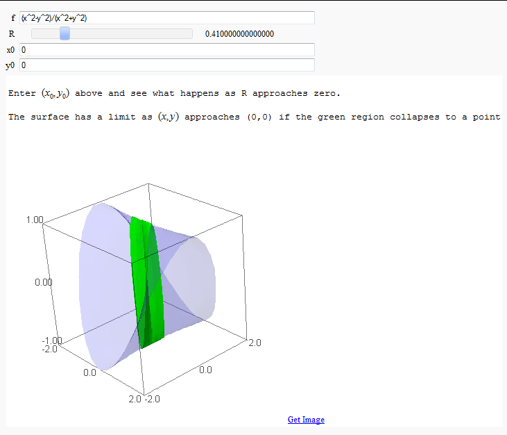
| html('Enter $(x_0 ,y_0 )$ above and see what happens as $ R \\rightarrow 0 $.') html('The surface has a limit as $(x,y) \\rightarrow $ ('+str(x0)+','+str(y0)+') if the green region collapses to a point.') |
pretty_print(html('Enter $(x_0 ,y_0 )$ above and see what happens as $ R \\rightarrow 0 $.')) pretty_print(html('The surface has a limit as $(x,y) \\rightarrow $ ('+str(x0)+','+str(y0)+') if the green region collapses to a point.')) |
| Line 1042: | Line 1042: |
| html('The red curves represent a couple of trajectories on the surface. If they do not meet, then') html('there is also no limit. (If computer hangs up, likely the computer can not do these limits.)') html('\n<center><font color="red">$\lim_{(x,?)\\rightarrow(x_0,y_0)} f(x,y) =%s$</font>'%str(limit_x)+' and <font color="red">$\lim_{(?,y)\\rightarrow(x_0,y_0)} f(x,y) =%s$</font></center>'%str(limit_y)) |
pretty_print(html('The red curves represent a couple of trajectories on the surface. If they do not meet, then')) pretty_print(html('there is also no limit. (If computer hangs up, likely the computer can not do these limits.)')) pretty_print(html('\n<center><font color="red">$\lim_{(x,?)\\rightarrow(x_0,y_0)} f(x,y) =%s$</font>'%str(limit_x)+' and <font color="red">$\lim_{(?,y)\\rightarrow(x_0,y_0)} f(x,y) =%s$</font></center>'%str(limit_y))) |
| Line 1081: | Line 1081: |
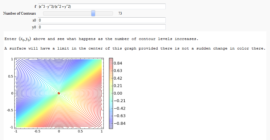
| html('Enter $(x_0 ,y_0 )$ above and see what happens as the number of contour levels $\\rightarrow \infty $.') html('A surface will have a limit in the center of this graph provided there is not a sudden change in color there.') |
pretty_print(html('Enter $(x_0 ,y_0 )$ above and see what happens as the number of contour levels $\\rightarrow \infty $.')) pretty_print(html('A surface will have a limit in the center of this graph provided there is not a sudden change in color there.')) |
| Line 1172: | Line 1172: |
| html(r'Function $ f(x,y)=%s$ '%latex(f(x,y))) | pretty_print(html(r'Function $ f(x,y)=%s$ '%latex(f(x,y)))) |
| Line 1186: | Line 1186: |
| html(r'<tr><td>$\quad f(%s,%s)\quad $</td><td>$\quad %s$</td>\ </tr>'%(latex(x0),latex(y0),z0.n())) |
pretty_print(html(r'<tr><td>$\quad f(%s,%s)\quad $</td><td>$\quad %s$</td>\ </tr>'%(latex(x0),latex(y0),z0.n()))) |
| Line 1220: | Line 1220: |
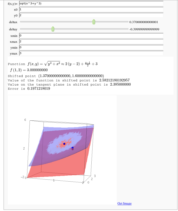
| html('Points x0 and y0 are values where the exact value of the function \ | pretty_print(html('Points x0 and y0 are values where the exact value of the function \ |
| Line 1222: | Line 1222: |
| and approximation by differential at shifted point are compared.') | and approximation by differential at shifted point are compared.')) |
| Line 1240: | Line 1240: |
| html(r'Function $ f(x,y)=%s \approx %s $ '%(latex(f(x,y)),latex(tangent(x,y)))) html(r' $f %s = %s$'%(latex((x0,y0)),latex(exact_value_ori))) html(r'Shifted point $%s$'%latex(((x0+deltax),(y0+deltay)))) html(r'Value of the function in shifted point is $%s$'%f(x0+deltax,y0+deltay)) html(r'Value on the tangent plane in shifted point is $%s$'%latex(approx_value)) html(r'Error is $%s$'%latex(abs_error)) |
pretty_print(html(r'Function $ f(x,y)=%s \approx %s $ '%(latex(f(x,y)),latex(tangent(x,y))))) pretty_print(html(r' $f %s = %s$'%(latex((x0,y0)),latex(exact_value_ori)))) pretty_print(html(r'Shifted point $%s$'%latex(((x0+deltax),(y0+deltay))))) pretty_print(html(r'Value of the function in shifted point is $%s$'%f(x0+deltax,y0+deltay))) pretty_print(html(r'Value on the tangent plane in shifted point is $%s$'%latex(approx_value))) pretty_print(html(r'Error is $%s$'%latex(abs_error))) |
| Line 1282: | Line 1282: |
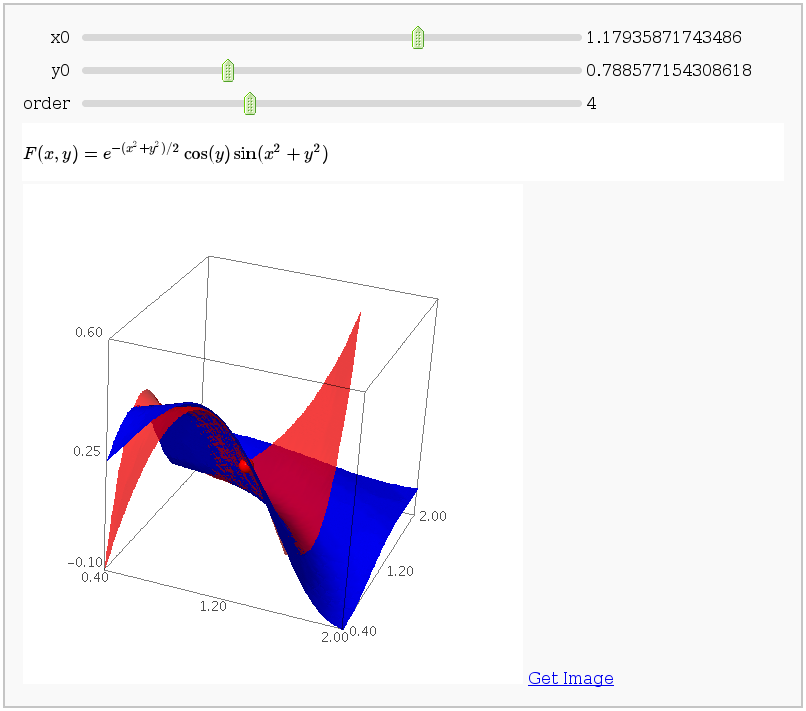
| html('$F(x,y) = e^{-(x^2+y^2)/2} \\cos(y) \\sin(x^2+y^2)$') | pretty_print(html('$F(x,y) = e^{-(x^2+y^2)/2} \\cos(y) \\sin(x^2+y^2)$')) |
| Line 1440: | Line 1440: |
| html(r'<font align=center size=+1>Lateral Surface $ \approx $ %s</font>'%str(line_integral_approx)) | pretty_print(html(r'<font align=center size=+1>Lateral Surface $ \approx $ %s</font>'%str(line_integral_approx))) |
| Line 1524: | Line 1524: |
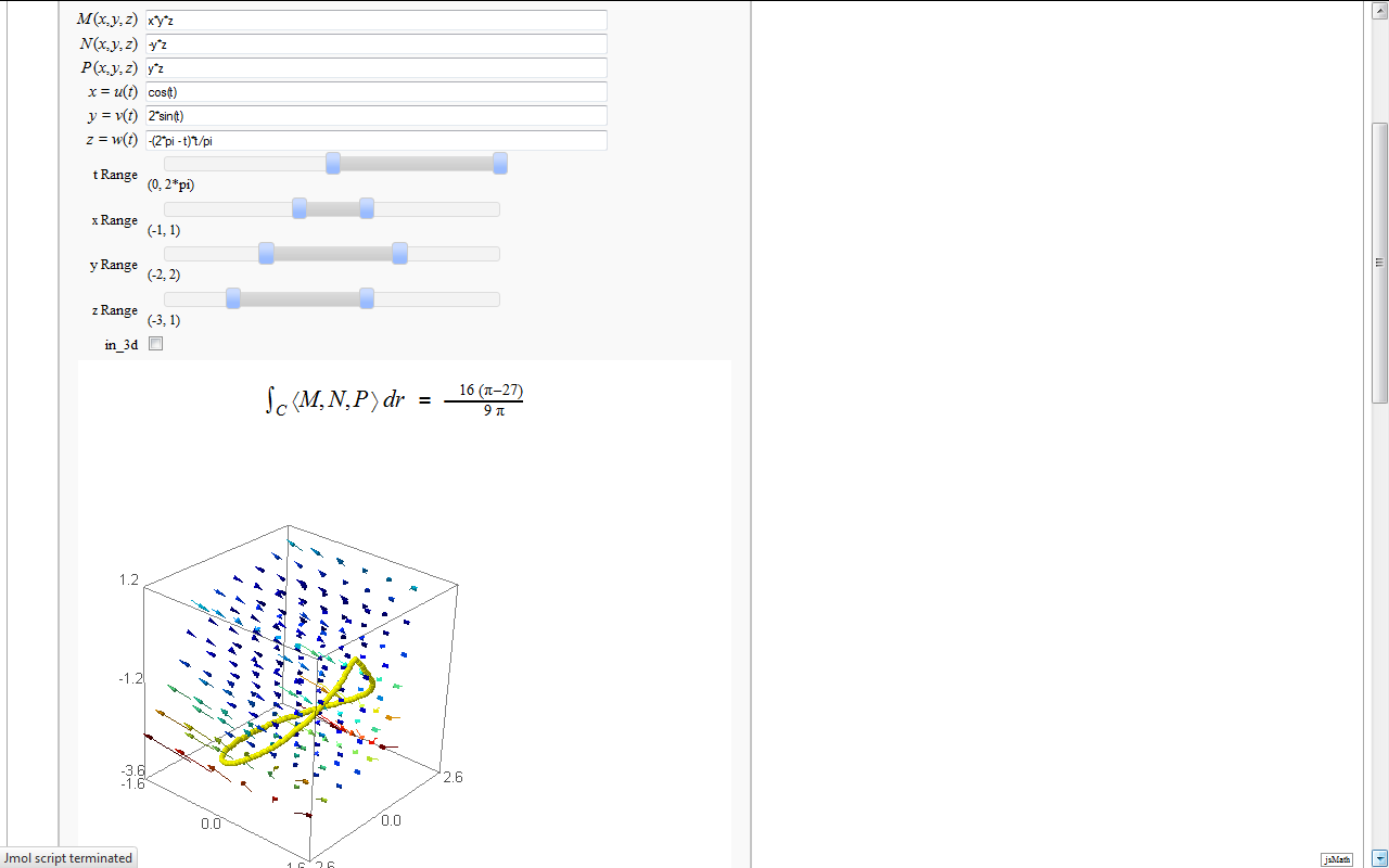
| html(r'<h2 align=center>$ \int_{C} \left \langle M,N,P \right \rangle dr $ = $ %s $ </h2>'%latex(line_integral)) | pretty_print(html(r'<h2 align=center>$ \int_{C} \left \langle M,N,P \right \rangle dr $ = $ %s $ </h2>'%latex(line_integral))) |
Sage Interactions - Calculus
goto interact main page
Contents
-
Sage Interactions - Calculus
- Root Finding Using Bisection
- Newton's Method
- A contour map and 3d plot of two inverse distance functions
- A simple tangent line grapher
- Numerical integrals with the midpoint rule
- Numerical integrals with various rules
- Some polar parametric curves
- Function tool
- Newton-Raphson Root Finding
- Coordinate Transformations (FIXME in Jupyter)
- Taylor Series
- Illustration of the precise definition of a limit
- A graphical illustration of sin(x)/x -> 1 as x-> 0
- Quadric Surface Plotter
- The midpoint rule for numerically integrating a function of two variables
- Gaussian (Legendre) quadrature
- Vector Calculus, 2-D Motion
- Vector Calculus, 3-D Motion (FIXME)
- Multivariate Limits by Definition
- Directional Derivatives
- 3D graph with points and curves
- Approximating function in two variables by differential
- Taylor approximations in two variables
- Volumes over non-rectangular domains
- Lateral Surface Area (FIXME in Jupyter)
- Parametric surface example (FIXME in Jupyter)
- Line Integrals in 3D Vector Field
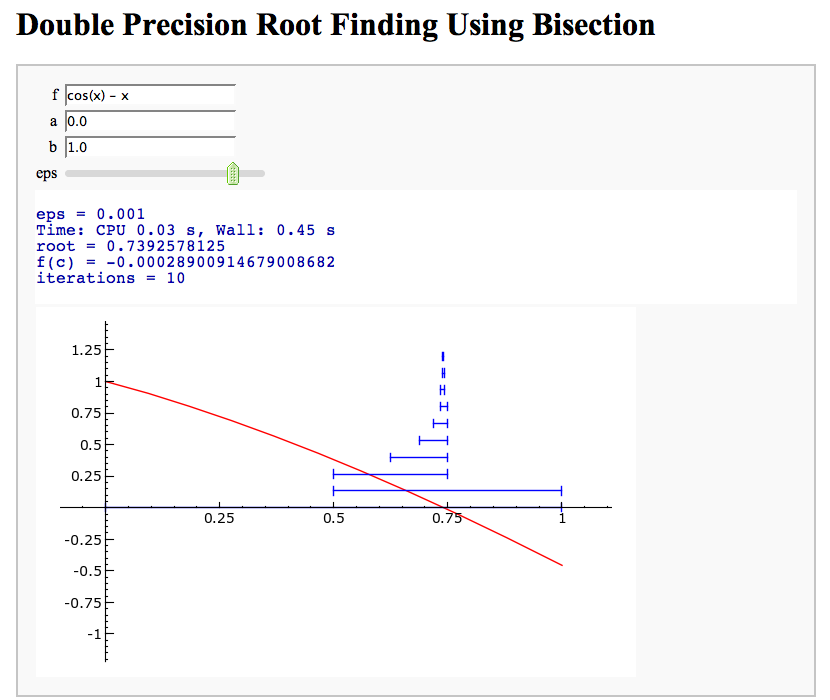
Root Finding Using Bisection
by William Stein
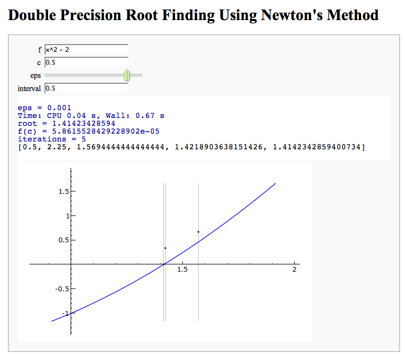
Newton's Method
Note that there is a more complicated Newton's method below.
by William Stein
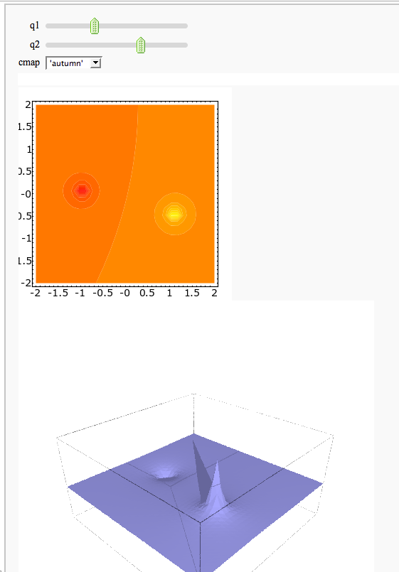
A contour map and 3d plot of two inverse distance functions
by William Stein
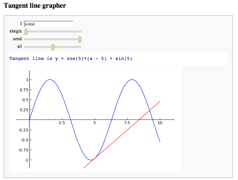
A simple tangent line grapher
by Marshall Hampton
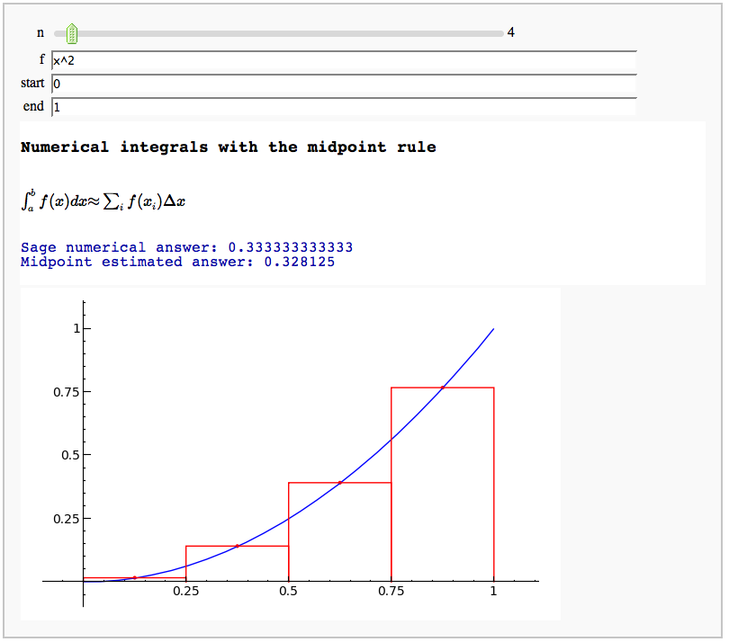
Numerical integrals with the midpoint rule
by Marshall Hampton
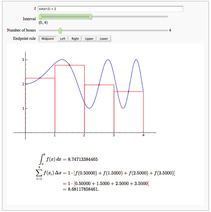
Numerical integrals with various rules
by Nick Alexander (based on the work of Marshall Hampton)
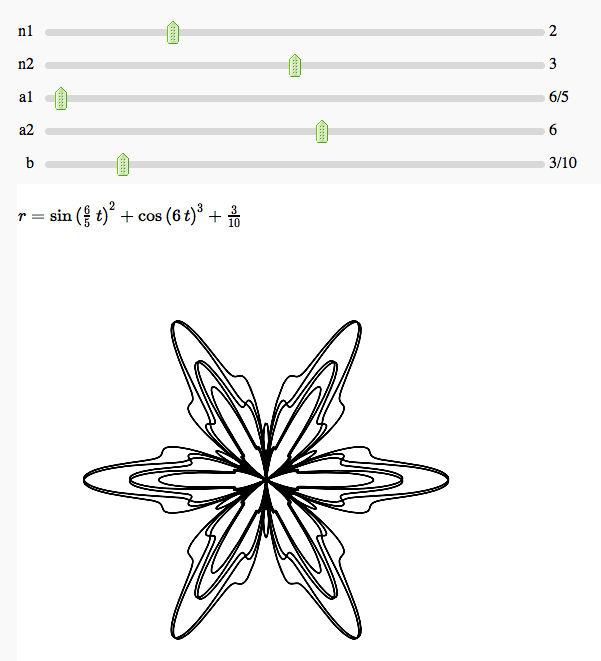
Some polar parametric curves
by Marshall Hampton. This is not very general, but could be modified to show other families of polar curves.
Function tool
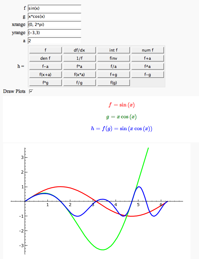
Enter symbolic functions f, g, and a, a range, then click the appropriate button to compute and plot some combination of f, g, and a along with f and g. This is inspired by the Matlab funtool GUI.
Newton-Raphson Root Finding
by Neal Holtz
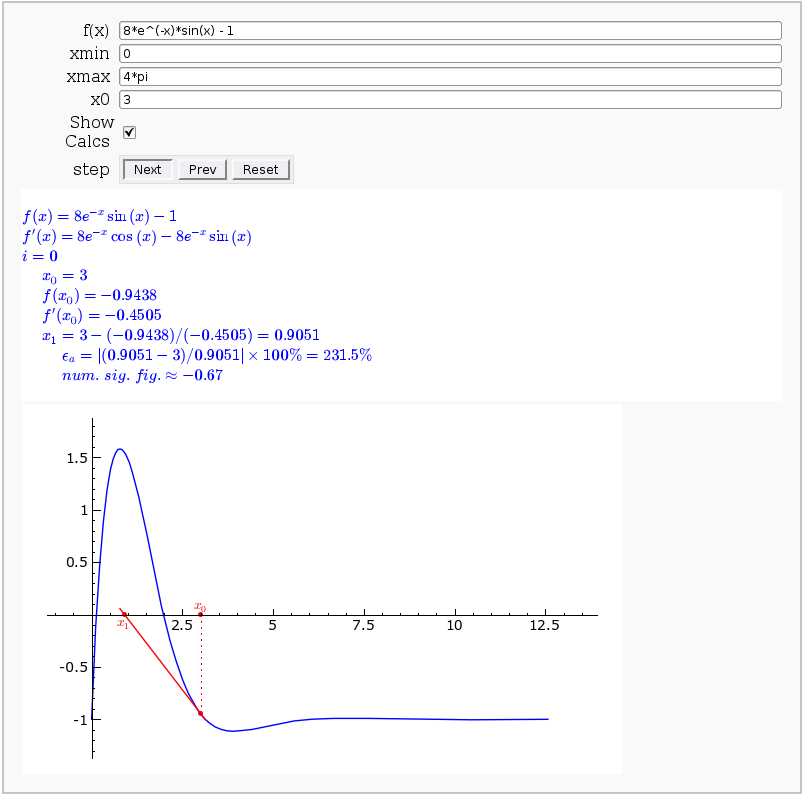
This allows user to display the Newton-Raphson procedure one step at a time. It uses the heuristic that, if any of the values of the controls change, then the procedure should be re-started, else it should be continued.
Coordinate Transformations (FIXME in Jupyter)
by Jason Grout
Taylor Series
by Harald Schilly
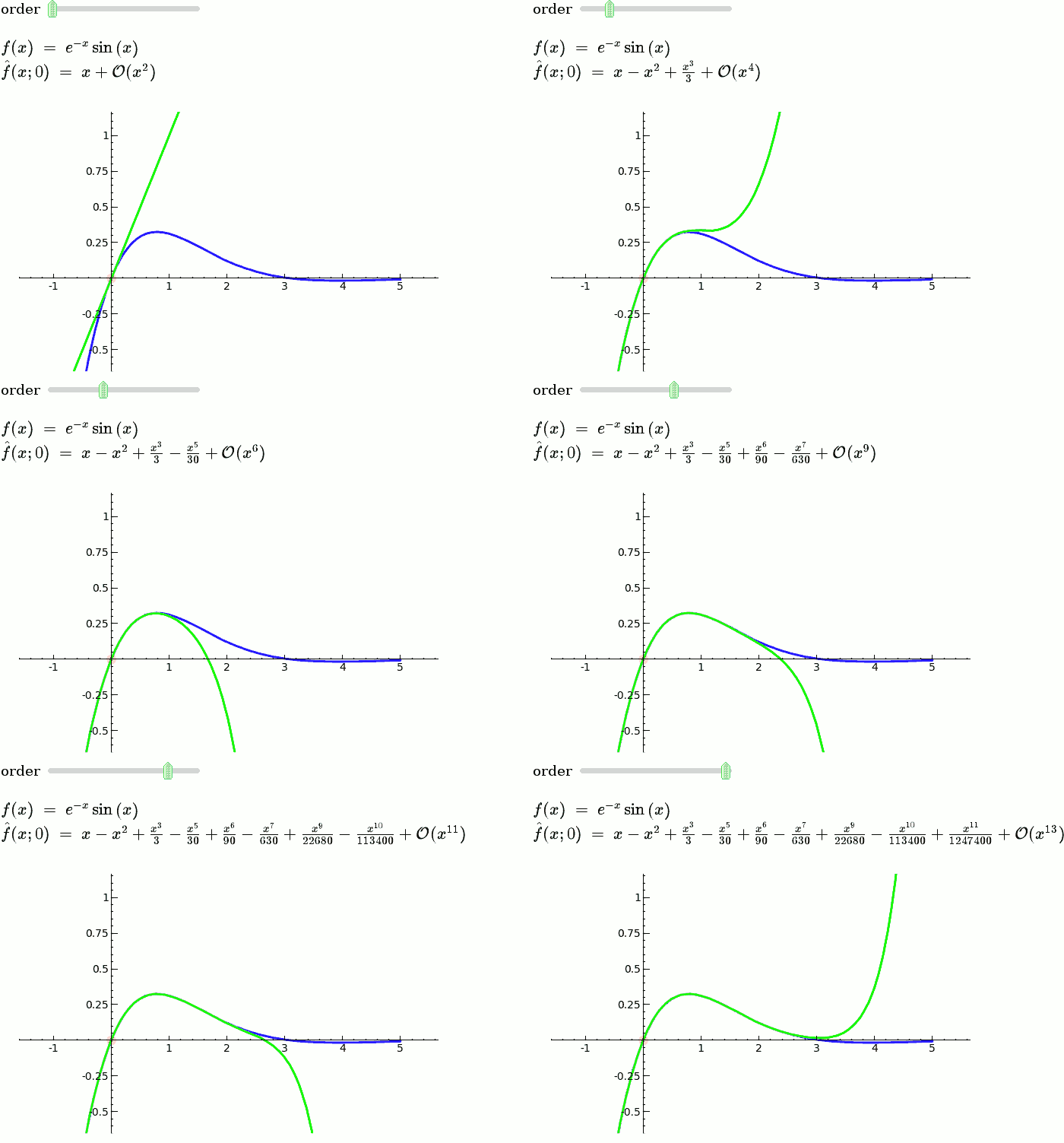
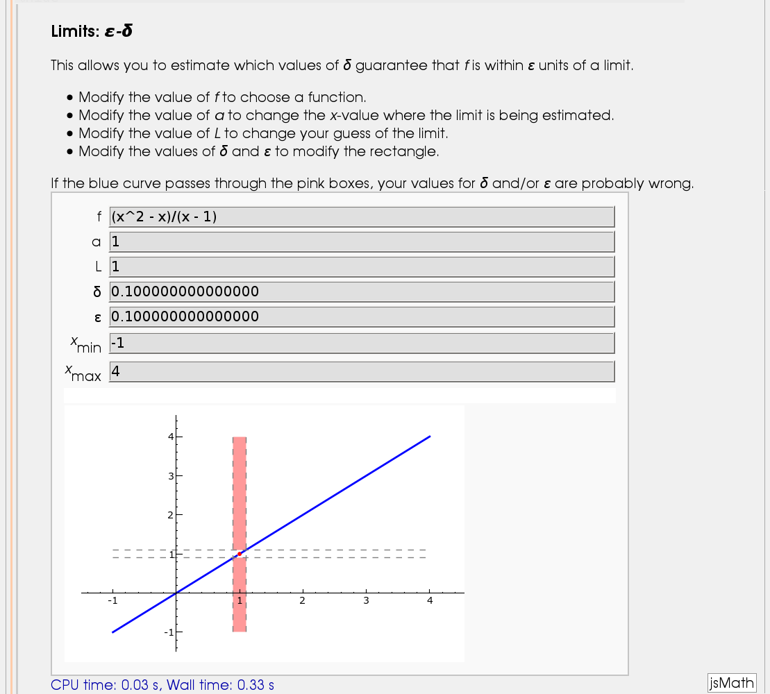
Illustration of the precise definition of a limit
by John Perry
I'll break tradition and put the image first. Apologies if this is Not A Good Thing.
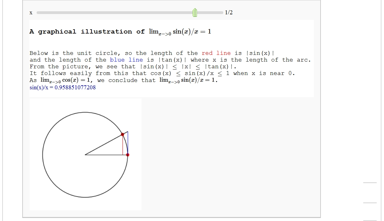
A graphical illustration of sin(x)/x -> 1 as x-> 0
by Wai Yan Pong
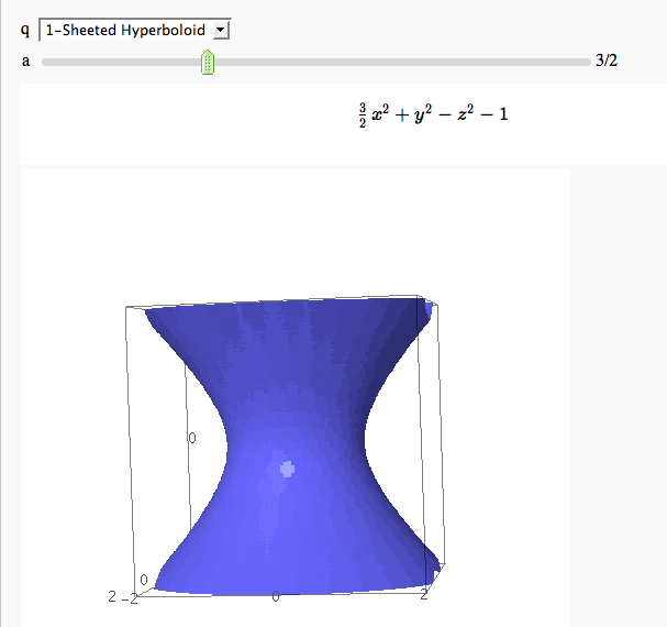
Quadric Surface Plotter
by Marshall Hampton. This is pretty simple, so I encourage people to spruce it up. In particular, it isn't set up to show all possible types of quadrics.
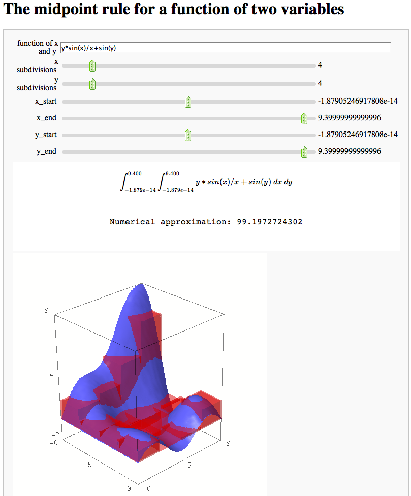
The midpoint rule for numerically integrating a function of two variables
by Marshall Hampton
Gaussian (Legendre) quadrature
by Jason Grout
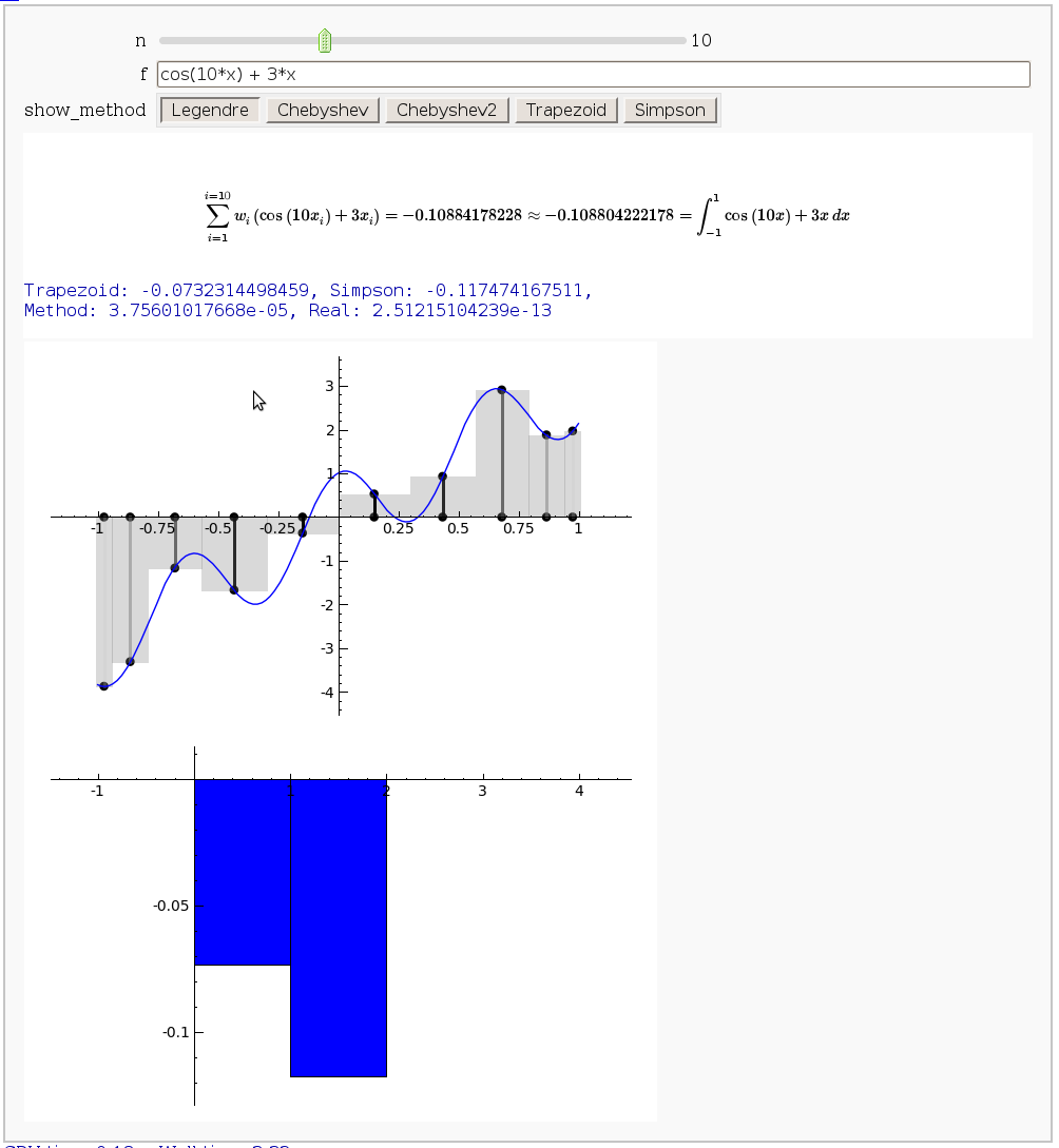
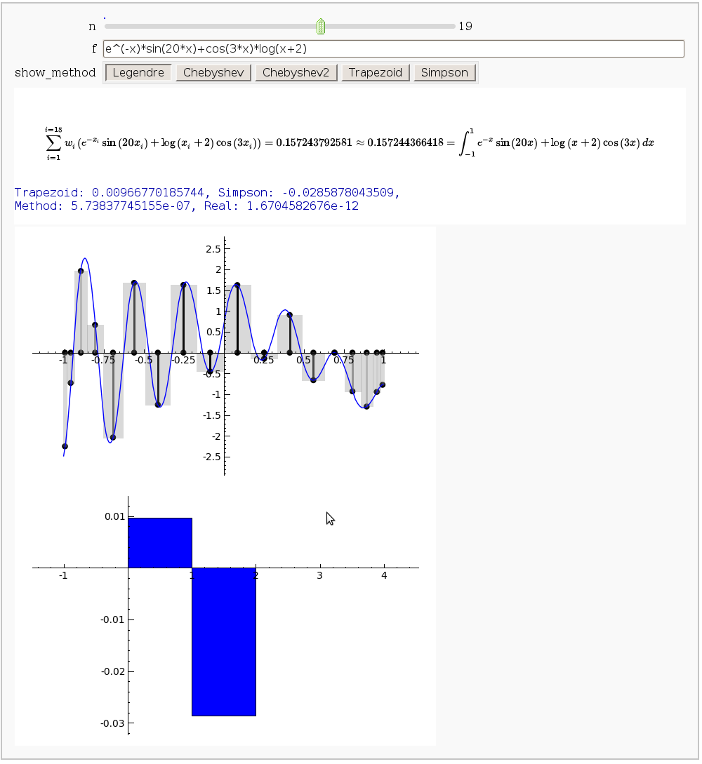
The output shows the points evaluated using Gaussian quadrature (using a weight of 1, so using Legendre polynomials). The vertical bars are shaded to represent the relative weights of the points (darker = more weight). The error in the trapezoid, Simpson, and quadrature methods is both printed out and compared through a bar graph. The "Real" error is the error returned from scipy on the definite integral.
Vector Calculus, 2-D Motion
By Rob Beezer
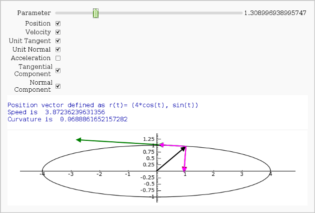
A fast_float() version is available in a worksheet
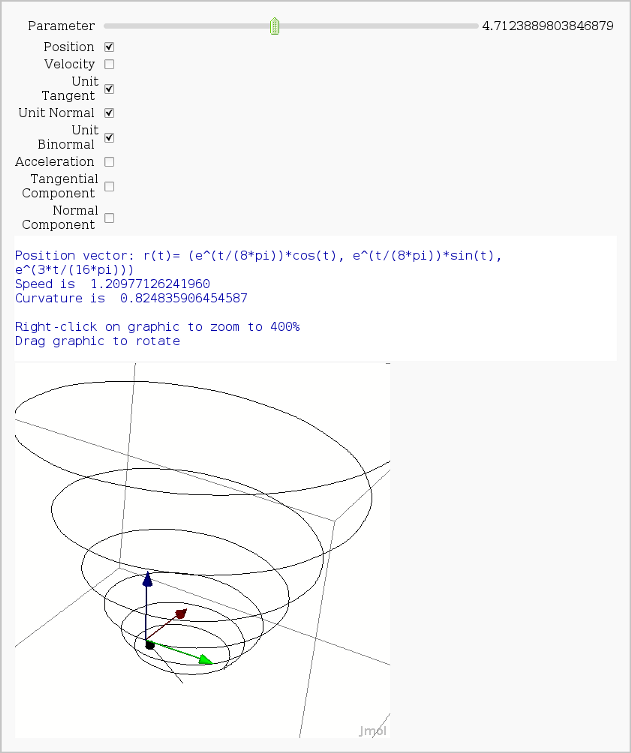
Vector Calculus, 3-D Motion (FIXME)
by Rob Beezer
Available as a worksheet
Multivariate Limits by Definition
by John Travis
http://sagenb.mc.edu/home/pub/97/
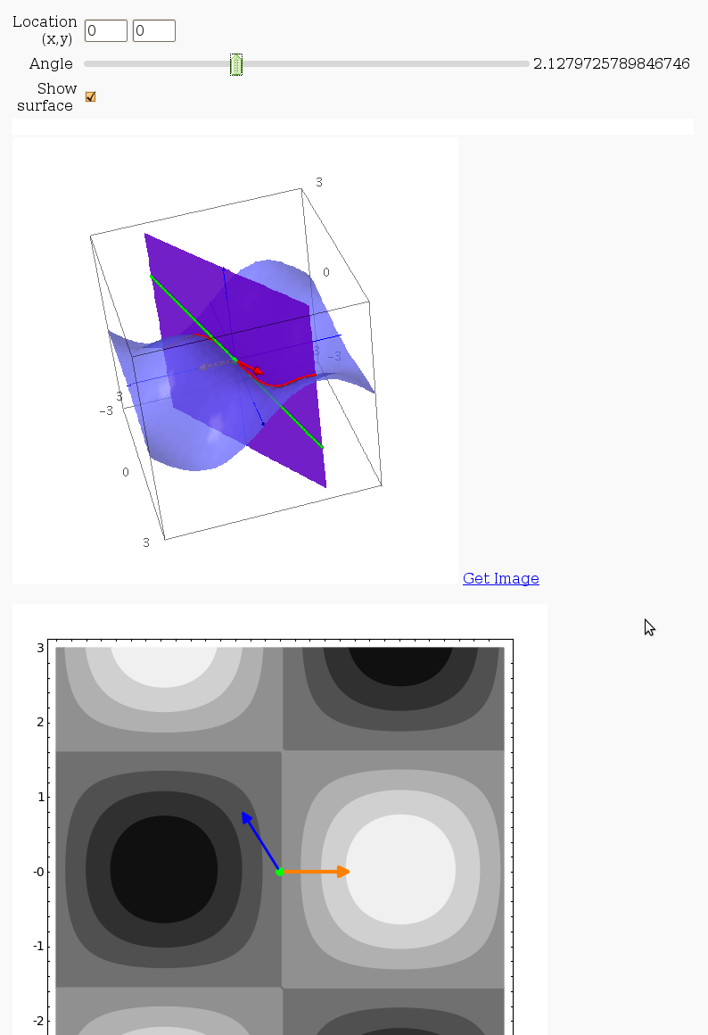
Directional Derivatives
This interact displays graphically a tangent line to a function, illustrating a directional derivative (the slope of the tangent line).
3D graph with points and curves
By Robert Marik
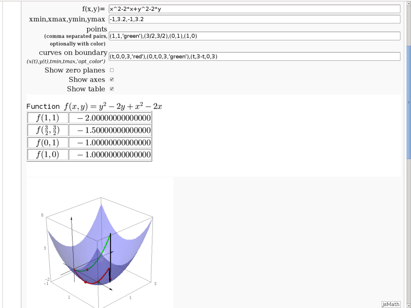
This sagelet is handy when showing local, constrained and absolute maxima and minima in two variables. Available as a worksheet
Approximating function in two variables by differential
by Robert Marik
Taylor approximations in two variables
by John Palmieri
This displays the nth order Taylor approximation, for n from 1 to 10, of the function sin(x2 + y2) cos(y) exp(-(x2+y2)/2).
Volumes over non-rectangular domains
by John Travis
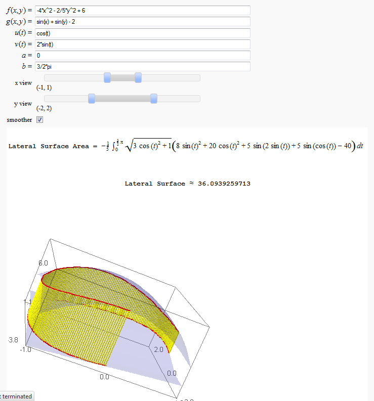
Lateral Surface Area (FIXME in Jupyter)
by John Travis
http://sagenb.mc.edu/home/pub/89/
Parametric surface example (FIXME in Jupyter)
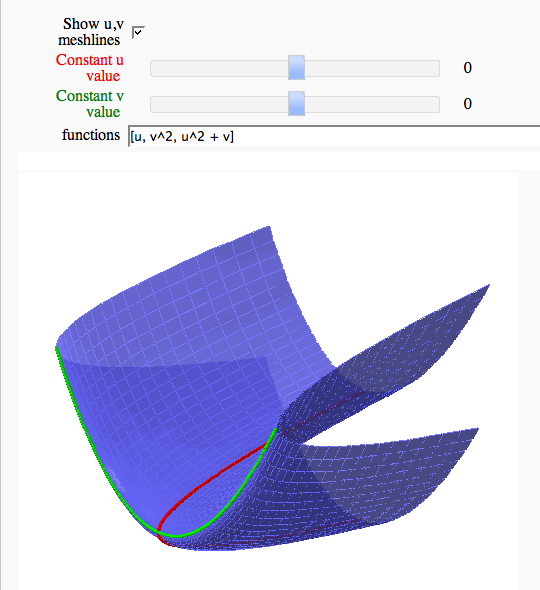
by Marshall Hampton
Line Integrals in 3D Vector Field
by John Travis
