|
Size: 7556
Comment: converted to 1.6 markup
|
← Revision 15 as of 2019-04-06 06:18:49 ⇥
Size: 7597
Comment: py3 print
|
| Deletions are marked like this. | Additions are marked like this. |
| Line 8: | Line 8: |
| {{{ | {{{#!sagecell |
| Line 20: | Line 20: |
| == 3D Groebner fan browser == | == 3D Groebner fan browser FIXME == |
| Line 22: | Line 22: |
| {{{ | {{{#!sagecell |
| Line 49: | Line 49: |
| print x.ieqs() + [[1,1,0,0,0],[1,0,1,0,0],[1,0,0,1,0],[1,0,0,0,1]] print x.linearities() print "" |
print(x.ieqs() + [[1,1,0,0,0],[1,0,1,0,0],[1,0,0,1,0],[1,0,0,0,1]]) print(x.linearities()) print("") |
| Line 58: | Line 58: |
| degs = [[max([q.degree(avar) for q in b]) for avar in our_vars] for b in a_gf.reduced_groebner_bases()] maxdegs = [max([float(q[i]) for q in degs]) for i in range(len(our_vars))] |
degs = [[max(q.degree(avar) for q in b) for avar in our_vars] for b in a_gf.reduced_groebner_bases()] maxdegs = [max(float(q[i]) for q in degs) for i in range(len(our_vars))] |
| Line 61: | Line 61: |
| color_list = [tuple([c[i]/max(c) for i in range(3)]) for c in color_list] | color_list = [tuple(c[i]/max(c) for i in range(3)) for c in color_list] |
| Line 79: | Line 79: |
| print cone_data._rays | print(cone_data._rays) |
| Line 99: | Line 99: |
| print id_gens | print(id_gens) |
| Line 116: | Line 116: |
| == Numerical Solutions of Polynomial Systems with PHCpack == | == Numerical Solutions of Polynomial Systems with PHCpack FIXME == |
| Line 119: | Line 119: |
| {{{ | {{{#!sagecell |
Sage Interactions - Algebra
goto interact main page
Contents
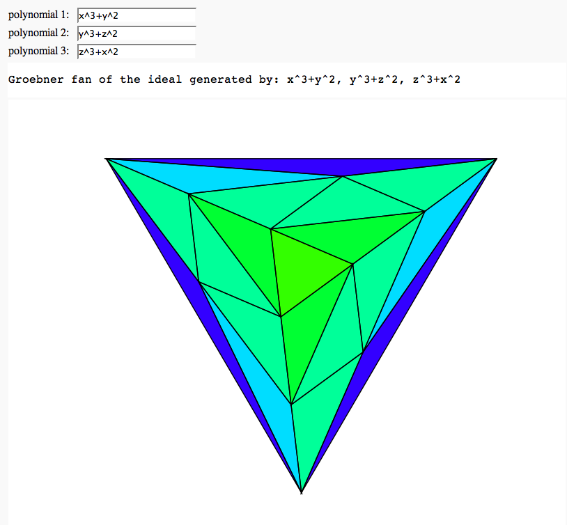
Groebner fan of an ideal
by Marshall Hampton; (needs sage-2.11 or higher, with gfan-0.3 interface)

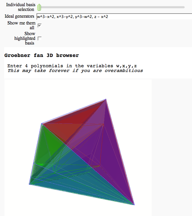
3D Groebner fan browser FIXME
by Marshall Hampton

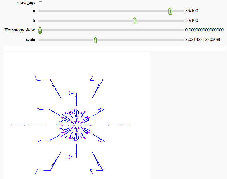
Numerical Solutions of Polynomial Systems with PHCpack FIXME
by Marshall Hampton; requires phcpack optional package (PHCpack written by Jan Verschelde). The example below is a two-parameter deformation of the cyclic-6 problem. Solution paths are tracked through the parameter homotopy.

