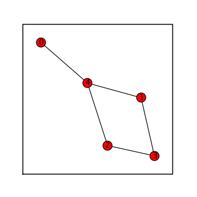
|
Size: 28083
Comment:
|
← Revision 28 as of 2008-11-14 13:41:50 ⇥
Size: 12645
Comment: converted to 1.6 markup
|
| Deletions are marked like this. | Additions are marked like this. |
| Line 1: | Line 1: |
| Gallery of Graph Generators in SAGE Emily Kirkman is working on this project. The goal of the Graph Generators Class is to implement constructors for many common graphs, as well as thorough docstrings that can be used for reference. The graph generators will grow as the Graph Theory Project does. So please check back for additions and feel free to leave requests in the suggestions section. We currently have 30 constructors of named graphs and basic structures. Most of these graphs are constructed with a preset dictionary of x-y coordinates of each node. This is advantagous SAGE graphs all have an associated graphics object, and examples of plotting options are shown on the graphs below. |
The Cayley graph for $A_5$: {{{ sage: G = sage.groups.perm_gps.permgroup.AlternatingGroup(5) sage: C = G.cayley_graph() sage: C.show3d(bgcolor=(0,0,0), arc_color=(1,1,1), vertex_size=0.02, arc_size=0.007, arc_size2=0.01, xres=1000, yres=800, iterations=200) }}} {{attachment:A5.jpg}} Emily Kirkman and Robert Miller are working on this project. [[http://wiki.sagemath.org/graph|Back to main wiki.]] The goal of the Graph Generators Class is to implement constructors for many common graphs, as well as thorough docstrings that can be used for reference. The graph generators will grow as the Graph Theory Project does. So please check back for additions and feel free to leave requests in the suggestions section. We currently have 54 constructors of named graphs and basic structures. Most of these graphs are constructed with a preset dictionary of x-y coordinates of each node. This is advantageous for both style and time. (The default graph plotting in SAGE uses the spring-layout algorithm). SAGE graphs all have an associated graphics object, and examples of plotting options are shown on the graphs below. |
| Line 11: | Line 19: |
| Due to the volume of graphs now in the generators class, this wiki page is now intended to give status updates and serve as a gallery of graphs currently implemented. To see information on a specific graph, run SAGE or the SAGE [http://sage.math.washington.edu:9001 notebook]. For a list of graph constructos, type "graphs." and hit tab. For docstrings, type the graph name and one question mark (i.e.: !"graphs.CubeGraph?") then shift + enter. For source code, do likewise with two question marks. The SAGE [http://sage.math.washington.edu:9001/graph Graph Theory Project] aims to implement Graph objects and algorithms in ["SAGE"]. [[TableOfContents]] |
Due to the volume of graphs now in the generators class, this wiki page is now intended to give status updates and serve as a gallery of graphs currently implemented. To see information on a specific graph, run SAGE or the SAGE [[http://sage.math.washington.edu:8100|notebook]]. For a list of graph constructors, type "graphs." and hit tab. For docstrings, type the graph name and one question mark (i.e.: "graphs.!CubeGraph?") then shift + enter. For source code, do likewise with two question marks. <<TableOfContents>> |
| Line 23: | Line 29: |
| * Bipartite Generators * Balanced tree * Dorogovstev golstev mendes graph * Grid (n-dim) * Hypercube * Chvatal * Desargues * Pappus * Sedgewick * Truncated cube * Truncated tetrahedron * Tutte * Also many more random generators and gens from degree sequence to sort through |
* Bipartite Generators * Grid (n-dim) * Sedgewick * Truncated cube * Truncated tetrahedron * Tutte |
| Line 47: | Line 46: |
| * Icosahedron | |
| Line 55: | Line 53: |
| = Currently Implemented in Graph Database = |
= Gallery of Graph Generators in SAGE = |
| Line 61: | Line 57: |
| === Chvatal Graph === {{{ sage: (graphs.ChvatalGraph()).show(figsize=[4,4], graph_border=True) }}} {{attachment:chvatal.png}} === Desargues Graph === {{{ sage: (graphs.DesarguesGraph()).show(figsize=[4,4], graph_border=True) }}} {{attachment:desargues.png}} === Flower Snark === {{{ sage: flower_snark = graphs.FlowerSnark() sage: flower_snark.set_boundary([15,16,17,18,19]) sage: flower_snark.show(figsize=[4,4], graph_border=True) }}} {{attachment:flower.png}} === Frucht === {{{ sage: frucht = graphs.FruchtGraph() sage: frucht.show(figsize=[4,4], graph_border=True) }}} {{attachment:frucht.png}} === Heawood === {{{ sage: heawood = graphs.HeawoodGraph() sage: heawood.show(figsize=[4,4], graph_border=True) }}} {{attachment:heawood.png}} === Möbius Kantor === {{{ sage: moebius_kantor = graphs.MoebiusKantorGraph() sage: moebius_kantor.show(figsize=[4,4], graph_border=True) }}} {{attachment:moebiuskantor.png}} === Pappus Graph === {{{ sage: (graphs.PappusGraph()).show(figsize=[4,4], graph_border=True) }}} {{attachment:pappus.png}} |
|
| Line 62: | Line 105: |
Info * The Petersen Graph is a named graph that consists of 10 vertices and 14 edges, usually drawn as a five-point star embedded in a pentagon. * The Petersen Graph is a common counterexample. For example, it is not Hamiltonian. Plotting * When plotting the Petersen graph with the spring-layout algorithm, we see that this graph is not very symmetric and thus the display may not be very meaningful. Efficiency of construction and plotting is not an issue, as the Petersen graph only has 10 vertices and 14 edges. * Our labeling convention here is to start on the outer pentagon from the top, moving counterclockwise. Then the nodes on the inner star, starting at the top and moving counterclockwise. Code {{{ pos_dict = {} for i in range(5): x = float(functions.cos(pi/2 + ((2*pi)/5)*i)) y = float(functions.sin(pi/2 + ((2*pi)/5)*i)) pos_dict[i] = [x,y] for i in range(10)[5:]: x = float(0.5*functions.cos(pi/2 + ((2*pi)/5)*i)) y = float(0.5*functions.sin(pi/2 + ((2*pi)/5)*i)) pos_dict[i] = [x,y] P = graph.Graph({0:[1,4,5], 1:[0,2,6], 2:[1,3,7], 3:[2,4,8], 4:[0,3,9],\ 5:[0,7,8], 6:[1,8,9], 7:[2,5,9], 8:[3,5,6], 9:[4,6,7]},\ pos=pos_dict, name="Petersen graph") return P }}} ==== Examples ==== Petersen Graph as constructed in this class: {{{ sage: petersen_this = graphs.PetersenGraph() sage: petersen_this.show() }}} attachment:petersen_pos.png Petersen Graph plotted using the spring layout algorithm: {{{ sage: petersen_spring = Graph({0:[1,4,5], 1:[0,2,6], 2:[1,3,7], 3:[2,4,8], 4:[0,3,9],\ 5:[0,7,8], 6:[1,8,9], 7:[2,5,9], 8:[3,5,6], 9:[4,6,7]}) sage: petersen_spring.show() }}} attachment:petersen_spring.png |
{{{ sage: petersen = graphs.PetersenGraph() sage: petersen.show(figsize=[4,4], graph_border=True) }}} {{attachment:petersen.png}} === Thomsen === {{{ sage: thomsen = graphs.ThomsenGraph() sage: thomsen.show(figsize=[4,4], graph_border=True) }}} {{attachment:thomsen.png}} |
| Line 106: | Line 120: |
| === Complete Bipartite Graphs === {{{ sage: comp_bip_list = [] sage: for i in range (2): ... for j in range (4): ... comp_bip_list.append(graphs.CompleteBipartiteGraph(i+3,j+1)) ... sage: graphs_list.show_graphs(comp_bip_list) }}} {{attachment:compbip.png}} |
|
| Line 107: | Line 132: |
Info * Returns a complete graph on n nodes. * A Complete Graph is a graph in which all nodes are connected to all other nodes. * This constructor is dependant on vertices numbered 0 through n-1 in NetworkX complete_graph() Plotting * Upon construction, the position dictionary is filled to override the spring-layout algorithm. By convention, each complete graph will be displayed with the first (0) node at the top, with the rest following in a counterclockwise manner. * In the complete graph, there is a big difference visually in using the spring-layout algorithm vs. the position dictionary used in this constructor. The position dictionary flattens the graph, making it clear which nodes an edge is connected to. But the complete graph offers a good example of how the spring-layout works. The edges push outward (everything is connected), causing the graph to appear as a 3-dimensional pointy ball. (See examples below). * Filling the position dictionary in advance adds O(n) to the constructor. Feel free to race the constructors below in the examples section. The much larger difference is the time added by the spring-layout algorithm when plotting. (Also shown in the example below). The spring model is typically described as O(n^3), as appears to be the case in the NetworkX source code. Code {{{ import networkx as NX pos_dict = {} for i in range(n): x = float(functions.cos((pi/2) + ((2*pi)/n)*i)) y = float(functions.sin((pi/2) + ((2*pi)/n)*i)) pos_dict[i] = [x,y] G = NX.complete_graph(n) return graph.Graph(G, pos=pos_dict, name="Complete graph on %d vertices"%n) }}} |
{{{ sage: comp_list = [] sage: for i in range(13)[1:]: ... comp_list.append(graphs.CompleteGraph(i)) ... sage: graphs_list.show_graphs(comp_list) }}} {{attachment:complete.png}} === Cube Graphs === {{{ sage: cube_list = [] sage: for i in range(6)[2:]: ... cube_list.append(graphs.CubeGraph(i)) ... sage: graphs_list.show_graphs(cube_list) }}} {{attachment:cube.png}} {{{ sage: bigger_cube = graphs.CubeGraph(8) sage: bigger_cube.show(figsize=[8,8], node_size=20, vertex_labels=False, graph_border=True) }}} {{attachment:biggercube.png}} === Balanced Tree === {{{ sage: (graphs.BalancedTree(3,5)).show(node_size=20, vertex_labels=False, figsize=[4,4], graph_border=True) }}} {{attachment:baltree.png}} === LCF Graph === {{{ sage: (graphs.LCFGraph(20, [-10,-7,-5,4,7,-10,-7,-4,5,7,-10,-7,6,-5,7,-10,-7,5,-6,7], 1)).show(figsize=[4,4], graph_border=True) }}} {{attachment:lcf.png}} == Platonic Solids == === Tetrahedral Graph === {{{ sage: tetrahedral = graphs.TetrahedralGraph() sage: tetrahedral.show(figsize=[4,4], graph_border=True) }}} {{attachment:tetrahedral.png}} === Hexahedral Graph === {{{ sage: (graphs.HexahedralGraph()).show(figsize=[4,4], graph_border=True) }}} {{attachment:hexahedral.png}} === Octahedral Graph === {{{ sage: octahedral = graphs.OctahedralGraph() sage: octahedral.show(figsize=[4,4], vertex_labels=False, node_size=50, graph_border=True) }}} {{attachment:octahedral.png}} === Icosahedral Graph === {{{ sage: (graphs.IcosahedralGraph()).show(figsize=[4,4], graph_border=True) }}} {{attachment:icosahedral.png}} === Dodecahedral Graph === {{{ sage: dodecahedral = graphs.DodecahedralGraph() sage: dodecahedral.show(figsize=[4,4], vertex_labels=False, node_size=50, graph_border=True) }}} {{attachment:dodecahedral.png}} == Pseudofractal Graphs == === Dorogovtsev Goltsev Mendes Graph === {{{ sage: (graphs.DorogovtsevGoltsevMendesGraph(5)).show(figsize=[4,4], graph_border=True, vertex_size=10, vertex_labels=False) }}} {{attachment:tmp_6.png}} |
| Line 134: | Line 215: |
Info * Returns a barbell graph with 2*n1 + n2 nodes. n1 must be greater than or equal to 2. * A barbell graph is a basic structure that consists of a path graph of order n2 connecting two complete graphs of order n1 each. * This constructor depends on NetworkX numeric labels. In this case, the (n1)th node connects to the path graph from one complete graph and the (n1+n2+1)th node connects to the path graph from the other complete graph. Plotting * Upon construction, the position dictionary is filled to override the spring-layout algorithm. By convention, each barbell graph will be displayed with the two complete graphs in the lower-left and upper-right corners, with the path graph connecting diagonally between the two. Thus the (n1)th node will be drawn at a 45 degree angle from the horizontal right center of the first complete graph, and the (n1+n2+1)th node will be drawn 45 degrees below the left horizontal center of the second complete graph. Code {{{ pos_dict = {} for i in range(n1): x = float(cos((pi/4) - ((2*pi)/n1)*i) - n2/2 - 1) y = float(sin((pi/4) - ((2*pi)/n1)*i) - n2/2 - 1) j = n1-1-i pos_dict[j] = [x,y] for i in range(n1+n2)[n1:]: x = float(i - n1 - n2/2 + 1) y = float(i - n1 - n2/2 + 1) pos_dict[i] = [x,y] for i in range(2*n1+n2)[n1+n2:]: x = float(cos((5*pi/4) + ((2*pi)/n1)*(i-n1-n2)) + n2/2 + 2) y = float(sin((5*pi/4) + ((2*pi)/n1)*(i-n1-n2)) + n2/2 + 2) pos_dict[i] = [x,y] import networkx G = networkx.barbell_graph(n1,n2) return graph.Graph(G, pos=pos_dict, name="Barbell graph") }}} ==== Examples ==== {{{ # Construct and show a barbell graph # Bar = 4, Bells = 9 sage: g = graphs.BarbellGraph(9,4) sage: g.show() }}} attachment here |
{{{ sage: barbell_list = [] sage: for i in range (4): ... for j in range (2): ... barbell_list.append(graphs.BarbellGraph(i+3, j+2)) ... sage: graphs_list.show_graphs(barbell_list) }}} {{attachment:barbell.png}} |
| Line 182: | Line 226: |
| Info * Returns a bull graph with 5 nodes. * A bull graph is named for its shape. It's a triangle with horns. * This constructor depends on NetworkX numeric labeling. Plotting * Upon construction, the position dictionary is filled to override the spring-layout algorithm. By convention, the bull graph is drawn as a triangle with the first node (0) on the bottom. The second and third nodes (1 and 2) complete the triangle. Node 3 is the horn connected to 1 and node 4 is the horn connected to node 2. Code {{{ pos_dict = [[0,0],[-1,1],[1,1],[-2,2],[2,2]] import networkx G = networkx.bull_graph() return graph.Graph(G, pos=pos_dict, name="Bull Graph") }}} ==== Examples ==== {{{ # Construct and show a bull graph sage: g = graphs.BullGraph() sage: g.show() }}} attachment here |
{{{ sage: bull = graphs.BullGraph() sage: bull.show(figsize=[4,4], graph_border=True) }}} {{attachment:bull.png}} |
| Line 214: | Line 233: |
Info * Returns a circular ladder graph with 2*n nodes. * A Circular ladder graph is a ladder graph that is connected at the ends, i.e.: a ladder bent around so that top meets bottom. Thus it can be described as two parrallel cycle graphs connected at each corresponding node pair. * This constructor depends on NetworkX numeric labels. Plotting * Upon construction, the position dictionary is filled to override the spring-layout algorithm. By convention, the circular ladder graph is displayed as an inner and outer cycle pair, with the first n nodes drawn on the inner circle. The first (0) node is drawn at the top of the inner-circle, moving clockwise after that. The outer circle is drawn with the (n+1)th node at the top, then counterclockwise as well. Code {{{ pos_dict = {} for i in range(n): x = float(cos((pi/2) + ((2*pi)/n)*i)) y = float(sin((pi/2) + ((2*pi)/n)*i)) pos_dict[i] = [x,y] for i in range(2*n)[n:]: x = float(2*(cos((pi/2) + ((2*pi)/n)*(i-n)))) y = float(2*(sin((pi/2) + ((2*pi)/n)*(i-n)))) pos_dict[i] = [x,y] import networkx G = networkx.circular_ladder_graph(n) return graph.Graph(G, pos=pos_dict, name="Circular Ladder graph") }}} ==== Examples ==== {{{ # Construct and show a circular ladder graph with 26 nodes sage: g = graphs.CircularLadderGraph(13) sage: g.show() }}} attachment here ADD SAGE LIST OF GRAPHS HERE INSTEAD {{{ # Create several circular ladder graphs in a SAGE graphics array sage: g = [] sage: j = [] sage: for i in range(9): ... k = graphs.CircularLadderGraph(i+3) ... g.append(k) ... sage: for i in range(3): ... n = [] ... for m in range(3): ... n.append(g[3*i + m].plot(node_size=50, vertex_labels=False)) ... j.append(n) ... sage: G = sage.plot.plot.GraphicsArray(j) sage: G.show() }}} attachment here |
{{{ sage: circ_ladder = graphs.CircularLadderGraph(9) sage: circ_ladder.show(figsize=[4,4], graph_border=True) }}} {{attachment:circladder.png}} === Claw Graph === {{{ sage: claw = graphs.ClawGraph() sage: claw.show(figsize=[4,4], graph_border=True) }}} {{attachment:claw.png}} |
| Line 274: | Line 247: |
Info * Returns a cycle graph with n nodes. * A cycle graph is a basic structure which is also typically called an n-gon. * This constructor is dependant on vertices numbered 0 through n-1 in NetworkX cycle_graph() Plotting * Upon construction, the position dictionary is filled to override the spring-layout algorithm. By convention, each cycle graph will be displayed with the first (0) node at the top, with the rest following in a counterclockwise manner. * The cycle graph is a good opportunity to compare efficiency of filling a position dictionary vs. using the spring-layout algorithm for plotting. Because the cycle graph is very symmetric, the resulting plots should be similar (in cases of small n). * Filling the position dictionary in advance adds O(n) to the constructor. Feel free to race the constructors below in the examples section. The much larger difference is the time added by the spring-layout algorithm when plotting. (Also shown in the example below). The spring model is typically described as O(n^3), as appears to be the case in the NetworkX source code. Code {{{ import networkx as NX pos_dict = {} for i in range(n): x = float(functions.cos((pi/2) + ((2*pi)/n)*i)) y = float(functions.sin((pi/2) + ((2*pi)/n)*i)) pos_dict[i] = [x,y] G = NX.cycle_graph(n) return graph.Graph(G, pos=pos_dict, name="Cycle graph on %d vertices"%n) }}} ==== Examples ==== The following examples require NetworkX (to use default): {{{ sage: import networkx as NX }}} Compare the constructor speeds. {{{ time n = NX.cycle_graph(3989); spring3989 = Graph(n) }}} CPU time: 0.05 s, Wall time: 0.07 s (Time results will vary.) {{{ time posdict3989 = graphs.CycleGraph(3989) }}} CPU time: 5.18 s, Wall time: 6.17 s (Time results will vary.) Compare the plotting speeds. {{{ sage: n = NX.cycle_graph(23) sage: spring23 = Graph(n) sage: posdict23 = graphs.CycleGraph(23) }}} {{{ time spring23.show() }}} CPU time: 2.04 s, Wall time: 2.72 s (Time results will vary.) attachment:cycle_spr23.png {{{ time posdict23.show() }}} CPU time: 0.57 s, Wall time: 0.71 s[[BR]] (Time results will vary.) attachment:cycl_pd23.png View many cycle graphs as a SAGE Graphics Array. With the position dictionary filled: ADD LIST HERE {{{ sage: g = [] sage: j = [] sage: for i in range(16): ... k = graphs.CycleGraph(i+3) ... g.append(k) ... sage: for i in range(4): ... n = [] ... for m in range(4): ... n.append(g[4*i + m].plot(node_size=50, vertex_labels=False)) ... j.append(n) ... sage: G = sage.plot.plot.GraphicsArray(j) sage: G.show() }}} attachment:cycle_pd_array.png With the spring-layout algorithm: ADD LIST HERE {{{ sage: g = [] sage: j = [] sage: for i in range(16): ... spr = NX.cycle_graph(i+3) ... k = Graph(spr) ... g.append(k) ... sage: for i in range(4): ... n = [] ... for m in range(4): ... n.append(g[4*i + m].plot(node_size=50, vertex_labels=False)) ... j.append(n) ... sage: G = sage.plot.plot.GraphicsArray(j) sage: G.show() }}} attachment:cycle_spr_array.png |
{{{ sage: cycle = graphs.CycleGraph(17) sage: cycle.show(figsize=[4,4], graph_border=True) }}} {{attachment:cycle.png}} |
| Line 392: | Line 254: |
Info * Returns a diamond graph with 4 nodes. * A diamond graph is a square with one pair of diagonal nodes connected. * This constructor depends on NetworkX numeric labeling. Plotting * Upon construction, the position dictionary is filled to override the spring-layout algorithm. By convention, the diamond graph is drawn as a diamond, with the first node on top, second on the left, third on the right, and fourth on the bottom; with the second and third node connected. Code {{{ pos_dict = [[0,1],[-1,0],[1,0],[0,-1]] import networkx G = networkx.diamond_graph() return graph.Graph(G, pos=pos_dict, name="Diamond Graph") }}} ==== Examples ==== {{{ # Construct and show a diamond graph sage: g = graphs.DiamondGraph() sage: g.show() }}} attachment here === Empty Graphs === Info * Returns an empty graph (0 nodes and 0 edges). * This is useful for constructing graphs by adding edges and vertices individually or in a loop. Plotting * When plotting, this graph will use the default spring-layout algorithm, unless a position dictionary is specified. Code {{{ return graph.Graph() }}} ==== Examples ==== Add one vertex to an empty graph. {{{ sage: empty1 = graphs.EmptyGraph() sage: empty1.add_vertex() sage: empty1.show() }}} attachment:empty1.png Use for loops to build a graph from an empty graph. {{{ sage: empty2 = graphs.EmptyGraph() sage: for i in range(5): ... empty2.add_vertex() # add 5 nodes, labeled 0-4 ... sage: for i in range(3): ... empty2.add_edge(i,i+1) # add edges {[0:1],[1:2],[2:3]} ... sage: for i in range(4)[1:]: ... empty2.add_edge(4,i) # add edges {[1:4],[2:4],[3:4]} ... sage: empty2.show() }}} attachment:empty2.png === Grid2d Graphs === Info * Returns a 2-dimensional grid graph with n1*n2 nodes (n1 rows and n2 columns). * A 2d grid graph resembles a 2 dimensional grid. All inner nodes are connected to their 4 neighbors. Outer (non-corner) nodes are connected to their 3 neighbors. Corner nodes are connected to their 2 neighbors. * This constructor depends on NetworkX numeric labels. Plotting * Upon construction, the position dictionary is filled to override the spring-layout algorithm. By convention, nodes are labelled in (row, column) pairs with (0, 0) in the top left corner. Edges will always be horizontal and vertical - another advantage of filling the position dictionary. Code {{{ pos_dict = {} for i in range(n1): y = -i for j in range(n2): x = j pos_dict[i,j] = [x,y] import networkx G = networkx.grid_2d_graph(n1,n2) return graph.Graph(G, pos=pos_dict, name="2D Grid Graph") }}} ==== Examples ==== {{{ # Construct and show a grid 2d graph # Rows = 5, Columns = 7 sage: g = graphs.Grid2dGraph(5,7) sage: g.show() }}} attachment here |
{{{ sage: diamond = graphs.DiamondGraph() sage: diamond.show(figsize=[4,4], graph_border=True) }}} {{attachment:diamond.png}} === Empty Graph === {{{ sage: empty = graphs.EmptyGraph() sage: empty.show(figsize=[1,1], graph_border=True) }}} {{attachment:empty.png}} === Grid 2d Graph === {{{ sage: grid = graphs.Grid2dGraph(3,5) sage: grid.show(figsize=[5,3]) }}} {{attachment:grid.png}} |
| Line 504: | Line 275: |
Info * Returns a house graph with 5 nodes. * A house graph is named for its shape. It is a triange (roof) over a square (walls). * This constructor depends on NetworkX numeric labeling. Plotting * Upon construction, the position dictionary is filled to override the spring-layout algorithm. By convention, the house graph is drawn with the first node in the lower-left corner of the house, the second in the lower-right corner of the house. The third node is in the upper-left corner connecting the roof to the wall, and the fourth is in the upper-right corner connecting the roof to the walll. The fifth node is the top of the roof, connected only to the third and fourth. Code ==== This has been updated! Change! ==== {{{ pos_dict = [[-1,0],[1,0],[-1,1],[1,1],[0,2]] import networkx G = networkx.house_graph() return graph.Graph(G, pos=pos_dict, name="House Graph") ==== Examples ==== {{{ # Construct and show a house graph sage: g = graphs.HouseGraph() sage: g.show() }}} attachment here |
{{{ sage: house = graphs.HouseGraph() sage: house.show(figsize=[4,4], graph_border=True) }}} {{attachment:house.png}} |
| Line 538: | Line 282: |
Info * Returns a house X graph with 5 nodes. * A house X graph is a house graph with two additional edges. The upper-right corner is connected to the lower-left. And the upper-left corner is connected to the lower-right. * This constructor depends on NetworkX numeric labeling. Plotting * Upon construction, the position dictionary is filled to override the spring-layout algorithm. By convention, the house X graph is drawn with the first node in the lower-left corner of the house, the second in the lower-right corner of the house. The third node is in the upper-left corner connecting the roof to the wall, and the fourth is in the upper-right corner connecting the roof to the walll. The fifth node is the top of the roof, connected only to the third and fourth. ==== Code, has been updated! ==== {{{ pos_dict = [[-1,0],[1,0],[-1,1],[1,1],[0,2]] import networkx G = networkx.house_x_graph() return graph.Graph(G, pos=pos_dict, name="House Graph") }}} ==== Examples ==== {{{ # Construct and show a house X graph sage: g = graphs.HouseXGraph() sage.: g.show() }}} attachment here |
{{{ sage: houseX = graphs.HouseXGraph() sage: houseX.show(figsize=[4,4], graph_border=True) }}} {{attachment:housex.png}} |
| Line 569: | Line 289: |
Info * Returns a Krackhardt kite graph with 10 nodes. * This constructor depends on NetworkX numeric labeling. * The Krackhardt kite graph was originally developed by David Krackhardt for the purpose of studying social networks. It is used to show the distinction between: degree centrality, betweeness centrality, and closeness centrality. For more information read the plotting section below in conjunction with the example. References * Kreps, V. (2002). "Social Network Analysis". [http://www.fsu.edu/~spap/water/network/intro.htm Link] Plotting * Upon construction, the position dictionary is filled to override the spring-layout algorithm. By convention, the graph is drawn left to right, in top to bottom row sequence of [2, 3, 2, 1, 1, 1] nodes on each row. This places the fourth node (3) in the center of the kite, with the highest degree. * But the fourth node only connects nodes that are otherwise connected, or those in its clique (i.e.: Degree Centrality). * The eigth (7) node is where the kite meets the tail. It has degree = 3, less than the average, but is the only connection between the kite and tail (i.e.: Betweenness Centrality). * The sixth and seventh nodes (5 and 6) are drawn in the third row and have degree = 5. These nodes have the shortest path to all other nodes in the graph (i.e.: Closeness Centrality). Please execute the example for visualization. Code {{{ pos_dict = [[-1,4],[1,4],[-2,3],[0,3],[2,3],[-1,2],[1,2],[0,1],[0,0],[0,-1]] import networkx G = networkx.krackhardt_kite_graph() return graph.Graph(G, pos=pos_dict, name="Krackhardt Kite Graph") }}} ==== Examples ==== {{{ # Construct and show a Krackhardt kite graph sage: g = graphs.KrackhardtKiteGraph() sage.: g.show() }}} attachment here |
{{{ sage: krackhardt = graphs.KrackhardtKiteGraph() sage: krackhardt.show(figsize=[4,4], graph_border=True) }}} {{attachment:krack.png}} |
| Line 607: | Line 296: |
| {{{ sage: ladder = graphs.LadderGraph(5) sage: ladder.show(figsize=[4,4], graph_border=True) }}} {{attachment:ladder.png}} |
|
| Line 609: | Line 303: |
| {{{ sage: lollipop_list = [] sage: for i in range (4): ... for j in range (2): ... lollipop_list.append(graphs.LollipopGraph(i+3, j+2)) ... sage: graphs_list.show_graphs(lollipop_list) }}} {{attachment:lollipop.png}} |
|
| Line 611: | Line 314: |
=== Star Graphs === Info * Returns a star graph with n+1 nodes. * A Star graph is a basic structure where one node is connected to all other nodes. * This constructor is dependant on NetworkX numeric labels. Plotting * Upon construction, the position dictionary is filled to override the spring-layout algorithm. By convention, each star graph will be displayed with the first (0) node in the center, the second node (1) at the top, with the rest following in a counterclockwise manner. (0) is the node connected to all other nodes. * The star graph is a good opportunity to compare efficiency of filling a position dictionary vs. using the spring-layout algorithm for plotting. As far as display, the spring-layout should push all other nodes away from the (0) node, and thus look very similar to this constructor's positioning. * Filling the position dictionary in advance adds O(n) to the constructor. Feel free to race the constructors below in the examples section. The much larger difference is the time added by the spring-layout algorithm when plotting. (Also shown in the example below). The spring model is typically described as O(n^3), as appears to be the case in the NetworkX source code. Code {{{ import networkx as NX pos_dict = {} pos_dict[0] = [0,0] for i in range(n+1)[1:]: x = float(functions.cos((pi/2) + ((2*pi)/n)*(i-1))) y = float(functions.sin((pi/2) + ((2*pi)/n)*(i-1))) pos_dict[i] = [x,y] G = NX.star_graph(n) return graph.Graph(G, pos=pos_dict, name="Star graph on %d vertices"%(n+1)) }}} ==== Examples ==== The following examples require NetworkX (to use default): {{{ sage: import networkx as NX }}} Compare the constructor speeds. {{{ time n = NX.star_graph(3989); spring3989 = Graph(n) }}} CPU time: 0.08 s, Wall time: 0.10 s (Time Results will vary.) {{{ time posdict3989 = graphs.StarGraph(3989) }}} CPU time: 5.43 s, Wall time: 7.41 s (Time results will vary.) Compare the plotting speeds. {{{ sage: n = NX.star_graph(23) sage: spring23 = Graph(n) sage: posdict23 = graphs.StarGraph(23) }}} {{{ time spring23.show() }}} CPU time: 2.31 s, Wall time: 3.14 s (Time results will vary.) attachment:star_spr23.png {{{ time posdict23.show() }}} CPU time: 0.68 s, Wall time: 0.80 s (Time results will vary.) attachment:star_pd23.png View many star graphs as a SAGE Graphics Array. ===== update to with list ===== With the position dictionary filled: {{{ sage: g = [] sage: j = [] sage: for i in range(16): ... k = graphs.StarGraph(i+3) ... g.append(k) ... sage: for i in range(4): ... n = [] ... for m in range(4): ... n.append(g[4*i + m].plot(node_size=50, vertex_labels=False)) ... j.append(n) ... sage: G = sage.plot.plot.GraphicsArray(j) sage: G.show() }}} attachment:star_array_pd.png With the spring-layout algorithm: ===== update with list ===== {{{ sage: g = [] sage: j = [] sage: for i in range(16): ... spr = NX.star_graph(i+3) ... k = Graph(spr) ... g.append(k) ... sage: for i in range(4): ... n = [] ... for m in range(4): ... n.append(g[4*i + m].plot(node_size=50, vertex_labels=False)) ... j.append(n) ... sage: G = sage.plot.plot.GraphicsArray(j) sage: G.show() }}} attachment:star_array_spr.png === Wheel Graphs === Info * Returns a Wheel graph with n nodes. * A Wheel graph is a basic structure where one node is connected to all other nodes and those (outer) nodes are connected cyclically. * This constructor depends on NetworkX numeric labels. Plotting * Upon construction, the position dictionary is filled to override the spring-layout algorithm. By convention, each wheel graph will be displayed with the first (0) node in the center, the second node at the top, and the rest following in a counterclockwise manner. * With the wheel graph, we see that it doesn't take a very large n at all for the spring-layout to give a counter-intuitive display. (See Graphics Array examples below). * Filling the position dictionary in advance adds O(n) to the constructor. Feel free to race the constructors below in the examples section. The much larger difference is the time added by the spring-layout algorithm when plotting. (Also shown in the example below). The spring model is typically described as O(n^3), as appears to be the case in the NetworkX source code. Code {{{ import networkx as NX pos_dict = {} pos_dict[0] = [0,0] for i in range(n)[1:]: x = float(functions.cos((pi/2) + ((2*pi)/(n-1))*(i-1))) y = float(functions.sin((pi/2) + ((2*pi)/(n-1))*(i-1))) pos_dict[i] = [x,y] G = NX.wheel_graph(n) return graph.Graph(G, pos=pos_dict, name="Wheel graph on %d vertices"%n) }}} ==== Examples ==== The following examples require NetworkX (to use default): {{{ sage: import networkx as NX }}} Compare the constructor speeds. {{{ time n = NX.wheel_graph(3989); spring3989 = Graph(n) }}} CPU time: 0.07 s, Wall time: 0.09 s (Time results will vary.) {{{ time posdict3989 = graphs.WheelGraph(3989) }}} CPU time: 5.99 s, Wall time: 8.74 s (Time results will vary.) Compare the plotting speeds. {{{ sage: n = NX.wheel_graph(23) sage: spring23 = Graph(n) sage: posdict23 = graphs.WheelGraph(23) }}} {{{ time spring23.show() }}} CPU time: 2.24 s, Wall time: 3.00 s (Time results will vary.) attachment:wheel_spr23.png {{{ time posdict23.show() }}} CPU time: 0.68 s, Wall time: 1.14 s (Time results will vary.) attachment:wheel_pd23.png View many wheel graphs as a SAGE Graphics Array. ===== update with list ===== With the position dictionary filled: {{{ sage: g = [] sage: j = [] sage: for i in range(16): ... k = graphs.WheelGraph(i+3) ... g.append(k) ... sage: for i in range(4): ... n = [] ... for m in range(4): ... n.append(g[4*i + m].plot(node_size=50, vertex_labels=False)) ... j.append(n) ... sage: G = sage.plot.plot.GraphicsArray(j) sage: G.show() }}} attachment:wheel_array_pd.png With the spring-layout algorithm: ===== update with list ===== {{{ sage: g = [] sage: j = [] sage: for i in range(16): ... spr = NX.wheel_graph(i+3) ... k = Graph(spr) ... g.append(k) ... sage: for i in range(4): ... n = [] ... for m in range(4): ... n.append(g[4*i + m].plot(node_size=50, vertex_labels=False)) ... j.append(n) ... sage: G = sage.plot.plot.GraphicsArray(j) sage: G.show() }}} attachment:wheel_array_spr.png |
{{{ sage: path_line = graphs.PathGraph(5) sage: path_circle = graphs.PathGraph(15) sage: path_maze = graphs.PathGraph(45) sage: path_list = [path_line, path_circle, path_maze] sage: graphs_list.show_graphs(path_list) }}} {{attachment:path.png}} === Star Graph === {{{ sage: star_list = [] sage: for i in range (12)[4:]: ... star_list.append(graphs.StarGraph(i)) ... sage: graphs_list.show_graphs(star_list) }}} {{attachment:star.png}} === Wheel Graph === {{{ sage: wheel_list = [] sage: for i in range (12)[4:]: ... wheel_list.append(graphs.WheelGraph(i)) ... sage: graphs_list.show_graphs(wheel_list) }}} {{attachment:wheel.png}} == Random Generators == === Random GNP === Use for dense graphs: {{{ time sage: (graphs.RandomGNP(16,.77)).show(figsize=[4,4], graph_border=True) }}} My results: CPU time: 0.74 s, Wall time: 0.73 s {{attachment:random.png}} === Random GNP Fast === Use for sparse graphs: {{{ time sage: (graphs.RandomGNPFast(16,.19)).show(figsize=[4,4], graph_border=True) }}} My results: CPU time: 0.63 s, Wall time: 0.62 s {{attachment:randomfast.png}} === Random Barabasi Albert === {{{ sage: (graphs.RandomBarabasiAlbert(7,3)).show(figsize=[4,4], graph_border=True) }}} {{attachment:barabasi.png}} === Random GNM === {{{ sage: (graphs.RandomGNM(7,16)).show(figsize=[4,4], graph_border=True) }}} {{attachment:gnm.png}} === Random Newman Watts Strogatz === {{{ sage: (graphs.RandomNewmanWattsStrogatz(7,3,.5)).show(figsize=[4,4], graph_border=True) }}} {{attachment:newman.png}} === Random Holme Kim === {{{ sage: (graphs.RandomHolmeKim(12,3,.4)).show(figsize=[4,4], graph_border=True) }}} {{attachment:holme.png}} === Random Lobster === {{{ sage: (graphs.RandomHolmeKim(12,3,.4)).show(figsize=[4,4], graph_border=True) }}} {{attachment:lobster.png}} === Random Tree Powerlaw === {{{ sage: (graphs.RandomTreePowerlaw(15)).show(figsize=[4,4], graph_border=True) }}} {{attachment:powerlaw.png}} === Random Regular === {{{ sage: (graphs.RandomRegular(3,20)).show(node_size=20, vertex_labels=False, figsize=[4,4], graph_border=True) }}} {{attachment:randreg.png}} === Random Shell === {{{ sage: (graphs.RandomShell([(10,20,0.8),(20,40,0.8)])).show(node_size=20, vertex_labels=False, figsize=[4,4], graph_border=True) }}} {{attachment:shell.png}} == Random Directed Graphs == === Random Directed GN === {{{ sage: (graphs.RandomDirectedGN(12)).show(node_size=20, vertex_labels=False, figsize=[4,4], graph_border=True) }}} {{attachment:randdirgn.png}} === Random Directed GNC === {{{ sage: (graphs.RandomDirectedGNC(12)).show(node_size=20, vertex_labels=False, figsize=[4,4], graph_border=True) }}} {{attachment:randdirgnc.png}} === Random Directed GNR === {{{ sage: (graphs.RandomDirectedGNR(12,.15)).show(node_size=20, vertex_labels=False, figsize=[4,4], graph_border=True) }}} {{attachment:randdirgnr.png}} == Graphs With a Given Degree Sequence == === Degree Sequence === {{{ sage: (graphs.DegreeSequence([3,3,3,3,3,3,3,3,3,3,3,3,3,3,3,3,3,3,3,3,3,3])).show(vertex_labels=False, node_size=30, figsize=[4,4], graph_border=True) }}} {{attachment:degseq.png}} === Degree Sequence Configuration Model === {{{ sage: (graphs.DegreeSequenceConfigurationModel([3,3,3,3,3,3,3,3,3,3,3,3,3,3,3,3,3,3,3,3])).show(vertex_labels=False, node_size=30, figsize=[4,4], graph_border=True) }}} {{attachment:degseqconf.png}} === Degree Sequence Tree === {{{ sage: (graphs.DegreeSequenceTree([3,1,3,3,1,1,1,2,1])).show(figsize=[4,4], graph_border=True) }}} {{attachment:degseqtree.png}} === Degree Sequence Expected === {{{ sage: (graphs.DegreeSequenceExpected([1,2,3,2,3])).show(figsize=[4,4],graph_border=True) }}} {{attachment:degseqexp.png}} |
The Cayley graph for A_5:
sage: G = sage.groups.perm_gps.permgroup.AlternatingGroup(5)
sage: C = G.cayley_graph()
sage: C.show3d(bgcolor=(0,0,0), arc_color=(1,1,1), vertex_size=0.02, arc_size=0.007, arc_size2=0.01, xres=1000, yres=800, iterations=200)
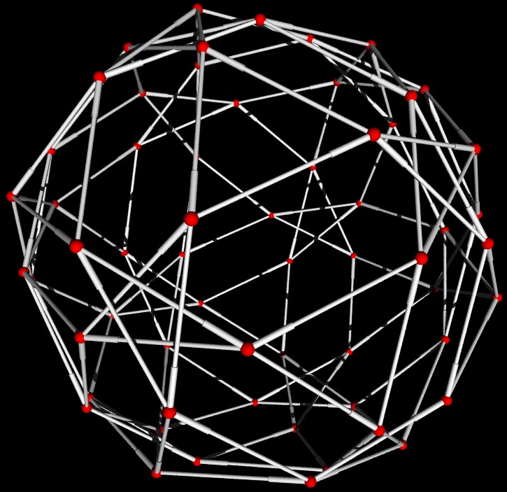
Emily Kirkman and Robert Miller are working on this project. Back to main wiki.
The goal of the Graph Generators Class is to implement constructors for many common graphs, as well as thorough docstrings that can be used for reference. The graph generators will grow as the Graph Theory Project does. So please check back for additions and feel free to leave requests in the suggestions section.
We currently have 54 constructors of named graphs and basic structures. Most of these graphs are constructed with a preset dictionary of x-y coordinates of each node. This is advantageous for both style and time. (The default graph plotting in SAGE uses the spring-layout algorithm). SAGE graphs all have an associated graphics object, and examples of plotting options are shown on the graphs below.
As we implement algorithms into the Graph Theory Package, the constructors of known graphs would set their properties upon instantiation as well. For example, if someone created a very large complete bipartite graph and then asked if it is a bipartite graph (not currently implemented), then instead of running through an algorithm to check it, we could return a value set at instantiation. Further, this will improve the reference use of the docstrings as we would list the properties of each named graph.
Due to the volume of graphs now in the generators class, this wiki page is now intended to give status updates and serve as a gallery of graphs currently implemented. To see information on a specific graph, run SAGE or the SAGE notebook. For a list of graph constructors, type "graphs." and hit tab. For docstrings, type the graph name and one question mark (i.e.: "graphs.CubeGraph?") then shift + enter. For source code, do likewise with two question marks.
Contents
Suggestions
- ???
Graphs I Plan to Add
Inherited from NetworkX
- Bipartite Generators
- Grid (n-dim)
- Sedgewick
- Truncated cube
- Truncated tetrahedron
- Tutte
Families of Graphs
- Generalized Petersen graphs
- Petersen Graph family
- Trees (Directed – not simple. Maybe Balanced tree constructor and query isTree)
- Cayley (Requires Edge Coloring)
- Paley
Named Graphs
- Brinkman
- Clebsch
- Grötzsch graph
- Tutte eight-cage
- Szekeres snark
- Thomassen graph
- Johnson (maybe own class)
- Turan
Gallery of Graph Generators in SAGE
Named Graphs
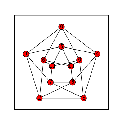
Chvatal Graph
sage: (graphs.ChvatalGraph()).show(figsize=[4,4], graph_border=True)
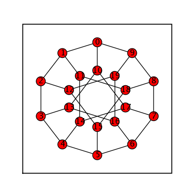
Desargues Graph
sage: (graphs.DesarguesGraph()).show(figsize=[4,4], graph_border=True)
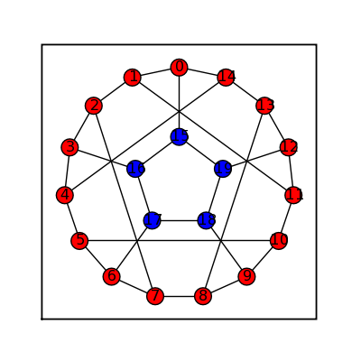
Flower Snark
sage: flower_snark = graphs.FlowerSnark()
sage: flower_snark.set_boundary([15,16,17,18,19])
sage: flower_snark.show(figsize=[4,4], graph_border=True)
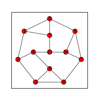
Frucht
sage: frucht = graphs.FruchtGraph()
sage: frucht.show(figsize=[4,4], graph_border=True)
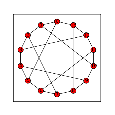
Heawood
sage: heawood = graphs.HeawoodGraph()
sage: heawood.show(figsize=[4,4], graph_border=True)
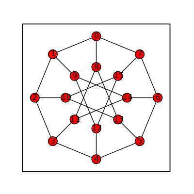
Möbius Kantor
sage: moebius_kantor = graphs.MoebiusKantorGraph()
sage: moebius_kantor.show(figsize=[4,4], graph_border=True)
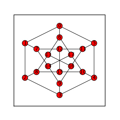
Pappus Graph
sage: (graphs.PappusGraph()).show(figsize=[4,4], graph_border=True)
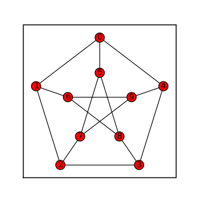
Petersen
sage: petersen = graphs.PetersenGraph()
sage: petersen.show(figsize=[4,4], graph_border=True)
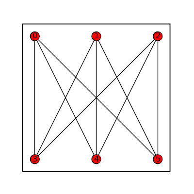
Thomsen
sage: thomsen = graphs.ThomsenGraph()
sage: thomsen.show(figsize=[4,4], graph_border=True)
Graph Families
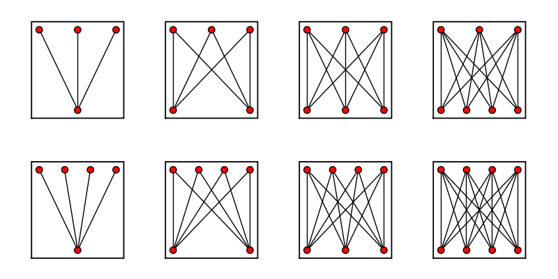
Complete Bipartite Graphs
sage: comp_bip_list = []
sage: for i in range (2):
... for j in range (4):
...  comp_bip_list.append(graphs.CompleteBipartiteGraph(i+3,j+1))
...
sage: graphs_list.show_graphs(comp_bip_list)
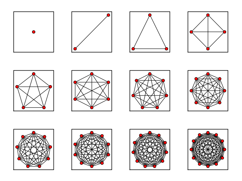
Complete Graphs
sage: comp_list = []
sage: for i in range(13)[1:]:
... comp_list.append(graphs.CompleteGraph(i))
...
sage: graphs_list.show_graphs(comp_list)
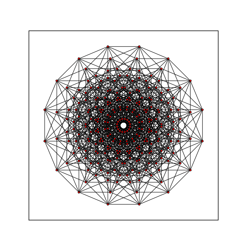
Cube Graphs
sage: cube_list = []
sage: for i in range(6)[2:]:
... cube_list.append(graphs.CubeGraph(i))
...
sage: graphs_list.show_graphs(cube_list)

sage: bigger_cube = graphs.CubeGraph(8)
sage: bigger_cube.show(figsize=[8,8], node_size=20, vertex_labels=False, graph_border=True)
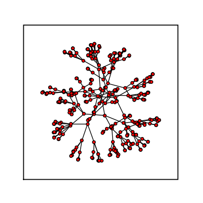
Balanced Tree
sage: (graphs.BalancedTree(3,5)).show(node_size=20, vertex_labels=False, figsize=[4,4], graph_border=True)
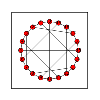
LCF Graph
sage: (graphs.LCFGraph(20, [-10,-7,-5,4,7,-10,-7,-4,5,7,-10,-7,6,-5,7,-10,-7,5,-6,7], 1)).show(figsize=[4,4], graph_border=True)
Platonic Solids
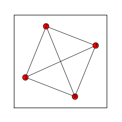
Tetrahedral Graph
sage: tetrahedral = graphs.TetrahedralGraph()
sage: tetrahedral.show(figsize=[4,4], graph_border=True)
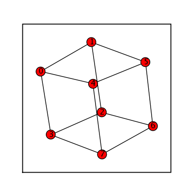
Hexahedral Graph
sage: (graphs.HexahedralGraph()).show(figsize=[4,4], graph_border=True)
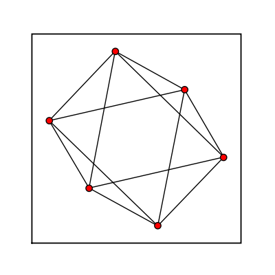
Octahedral Graph
sage: octahedral = graphs.OctahedralGraph()
sage: octahedral.show(figsize=[4,4], vertex_labels=False, node_size=50, graph_border=True)
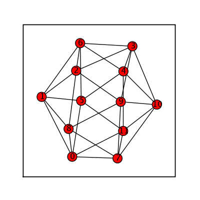
Icosahedral Graph
sage: (graphs.IcosahedralGraph()).show(figsize=[4,4], graph_border=True)
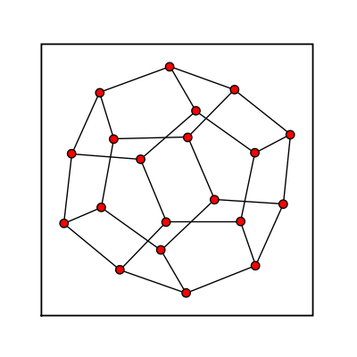
Dodecahedral Graph
sage: dodecahedral = graphs.DodecahedralGraph()
sage: dodecahedral.show(figsize=[4,4], vertex_labels=False, node_size=50, graph_border=True)
Pseudofractal Graphs
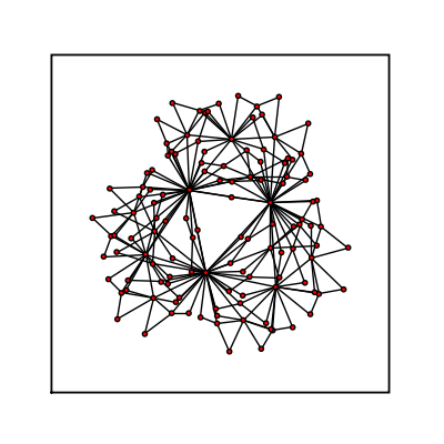
Dorogovtsev Goltsev Mendes Graph
sage: (graphs.DorogovtsevGoltsevMendesGraph(5)).show(figsize=[4,4], graph_border=True, vertex_size=10, vertex_labels=False)
Basic Structures
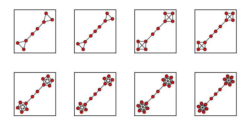
Barbell Graph
sage: barbell_list = []
sage: for i in range (4):
... for j in range (2):
...  barbell_list.append(graphs.BarbellGraph(i+3, j+2))
...
sage: graphs_list.show_graphs(barbell_list)
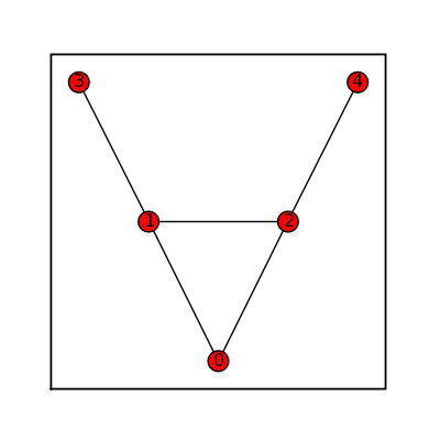
Bull Graph
sage: bull = graphs.BullGraph()
sage: bull.show(figsize=[4,4], graph_border=True)
Circular Ladder Graph
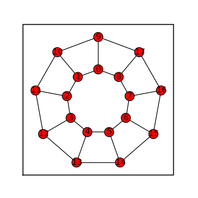
sage: circ_ladder = graphs.CircularLadderGraph(9)
sage: circ_ladder.show(figsize=[4,4], graph_border=True)
Claw Graph
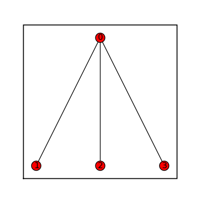
sage: claw = graphs.ClawGraph()
sage: claw.show(figsize=[4,4], graph_border=True)
Cycle Graphs
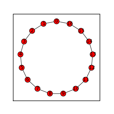
sage: cycle = graphs.CycleGraph(17)
sage: cycle.show(figsize=[4,4], graph_border=True)
Diamond Graph
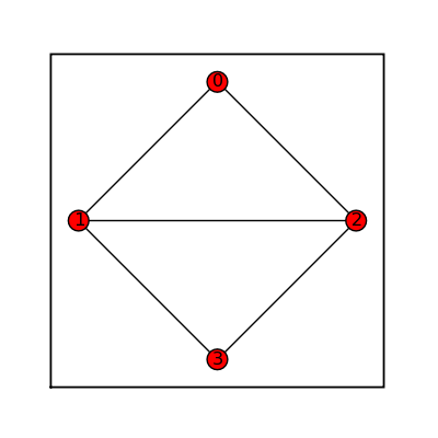
sage: diamond = graphs.DiamondGraph()
sage: diamond.show(figsize=[4,4], graph_border=True)
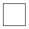
Empty Graph
sage: empty = graphs.EmptyGraph()
sage: empty.show(figsize=[1,1], graph_border=True)
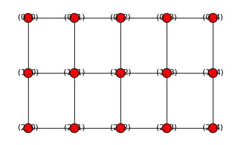
Grid 2d Graph
sage: grid = graphs.Grid2dGraph(3,5)
sage: grid.show(figsize=[5,3])
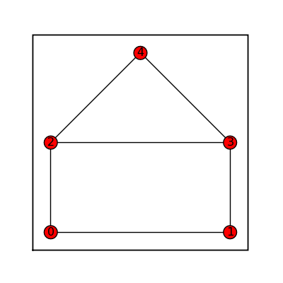
House Graph
sage: house = graphs.HouseGraph()
sage: house.show(figsize=[4,4], graph_border=True)
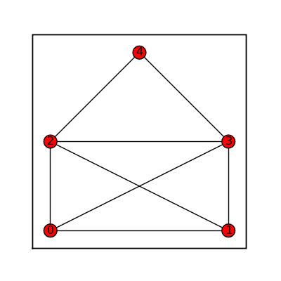
House X Graph
sage: houseX = graphs.HouseXGraph()
sage: houseX.show(figsize=[4,4], graph_border=True)
Krackhardt Kite Graph
sage: krackhardt = graphs.KrackhardtKiteGraph()
sage: krackhardt.show(figsize=[4,4], graph_border=True)
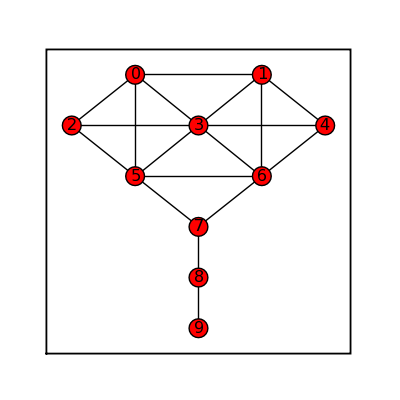
Ladder Graph
sage: ladder = graphs.LadderGraph(5)
sage: ladder.show(figsize=[4,4], graph_border=True)
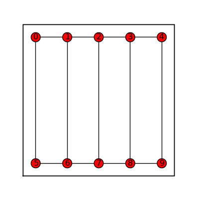
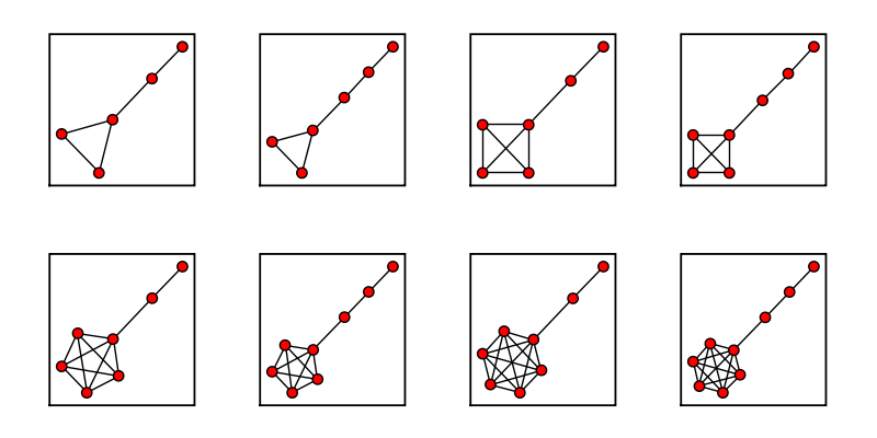
Lollipop Graph
sage: lollipop_list = []
sage: for i in range (4):
... for j in range (2):
...  lollipop_list.append(graphs.LollipopGraph(i+3, j+2))
...
sage: graphs_list.show_graphs(lollipop_list)
Path Graph
sage: path_line = graphs.PathGraph(5)
sage: path_circle = graphs.PathGraph(15)
sage: path_maze = graphs.PathGraph(45)
sage: path_list = [path_line, path_circle, path_maze]
sage: graphs_list.show_graphs(path_list)

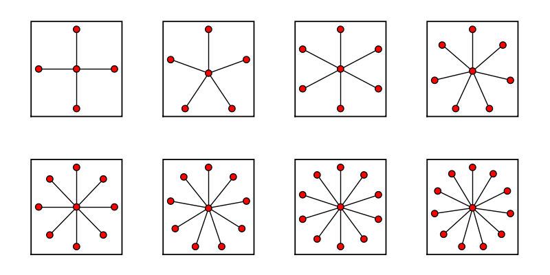
Star Graph
sage: star_list = []
sage: for i in range (12)[4:]:
... star_list.append(graphs.StarGraph(i))
...
sage: graphs_list.show_graphs(star_list)
Wheel Graph
sage: wheel_list = []
sage: for i in range (12)[4:]:
... wheel_list.append(graphs.WheelGraph(i))
...
sage: graphs_list.show_graphs(wheel_list)
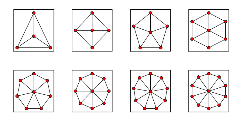
Random Generators
Random GNP
Use for dense graphs:
time
sage: (graphs.RandomGNP(16,.77)).show(figsize=[4,4], graph_border=True)
My results: CPU time: 0.74 s, Wall time: 0.73 s 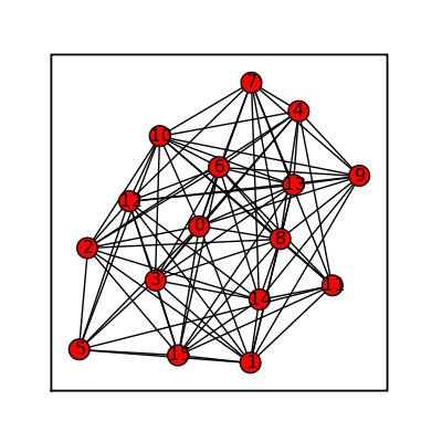
Random GNP Fast
Use for sparse graphs:
time
sage: (graphs.RandomGNPFast(16,.19)).show(figsize=[4,4], graph_border=True)
My results: CPU time: 0.63 s, Wall time: 0.62 s 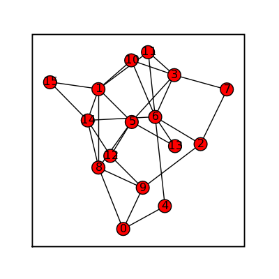
Random Barabasi Albert
sage: (graphs.RandomBarabasiAlbert(7,3)).show(figsize=[4,4], graph_border=True)
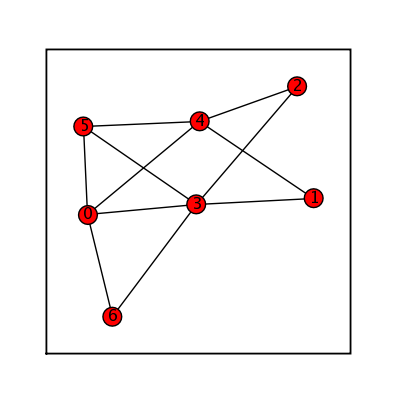
Random GNM
sage: (graphs.RandomGNM(7,16)).show(figsize=[4,4], graph_border=True)
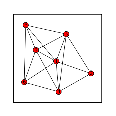
Random Newman Watts Strogatz
sage: (graphs.RandomNewmanWattsStrogatz(7,3,.5)).show(figsize=[4,4], graph_border=True)
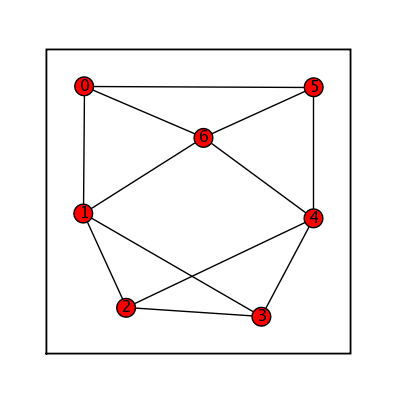
Random Holme Kim
sage: (graphs.RandomHolmeKim(12,3,.4)).show(figsize=[4,4], graph_border=True)
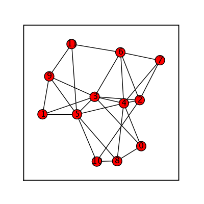
Random Lobster
sage: (graphs.RandomHolmeKim(12,3,.4)).show(figsize=[4,4], graph_border=True)
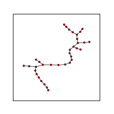
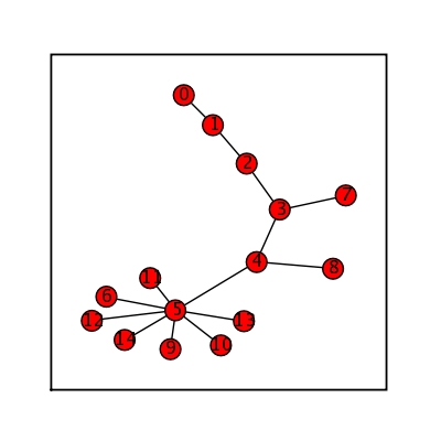
Random Tree Powerlaw
sage: (graphs.RandomTreePowerlaw(15)).show(figsize=[4,4], graph_border=True)
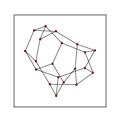
Random Regular
sage: (graphs.RandomRegular(3,20)).show(node_size=20, vertex_labels=False, figsize=[4,4], graph_border=True)
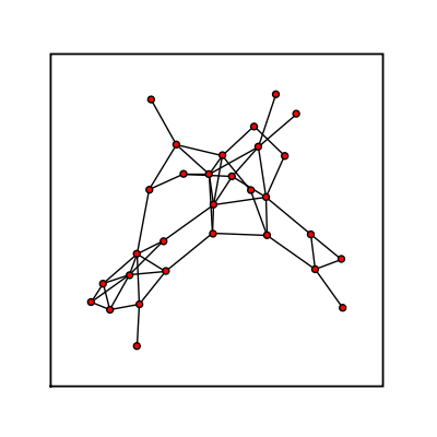
Random Shell
sage: (graphs.RandomShell([(10,20,0.8),(20,40,0.8)])).show(node_size=20, vertex_labels=False, figsize=[4,4], graph_border=True)
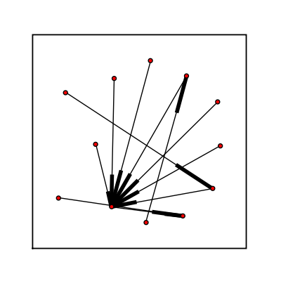
Random Directed Graphs
Random Directed GN
sage: (graphs.RandomDirectedGN(12)).show(node_size=20, vertex_labels=False, figsize=[4,4], graph_border=True)
Random Directed GNC
sage: (graphs.RandomDirectedGNC(12)).show(node_size=20, vertex_labels=False, figsize=[4,4], graph_border=True)
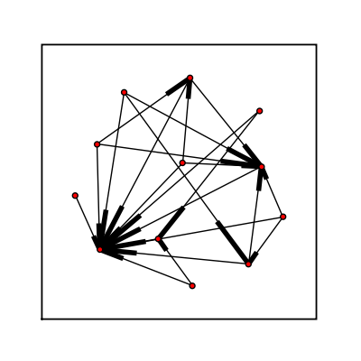
Random Directed GNR
sage: (graphs.RandomDirectedGNR(12,.15)).show(node_size=20, vertex_labels=False, figsize=[4,4], graph_border=True)
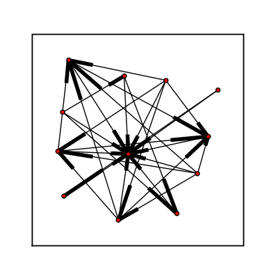
Graphs With a Given Degree Sequence
Degree Sequence
sage: (graphs.DegreeSequence([3,3,3,3,3,3,3,3,3,3,3,3,3,3,3,3,3,3,3,3,3,3])).show(vertex_labels=False, node_size=30, figsize=[4,4], graph_border=True)
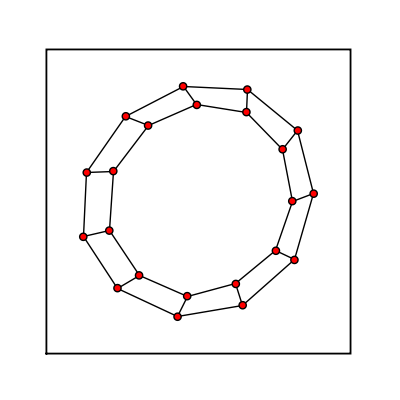
Degree Sequence Configuration Model
sage: (graphs.DegreeSequenceConfigurationModel([3,3,3,3,3,3,3,3,3,3,3,3,3,3,3,3,3,3,3,3])).show(vertex_labels=False, node_size=30, figsize=[4,4], graph_border=True)
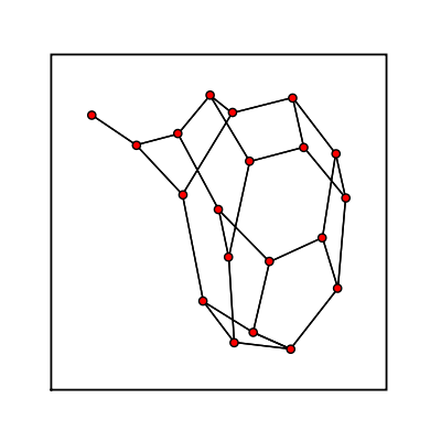
Degree Sequence Tree
sage: (graphs.DegreeSequenceTree([3,1,3,3,1,1,1,2,1])).show(figsize=[4,4], graph_border=True)
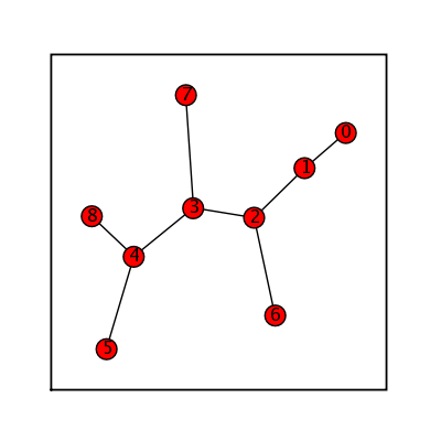
Degree Sequence Expected
sage: (graphs.DegreeSequenceExpected([1,2,3,2,3])).show(figsize=[4,4],graph_border=True)
