see the attachments
This page contains animations drawn using Sage. One can create an animation (.gif) in Sage from a list of graphics objects using the animate command. Currently, to export an animation in .gif format, you might need to install the ImageMagick command line tools package (the convert command). See the documentation for more information:
sage: animate?
Contents
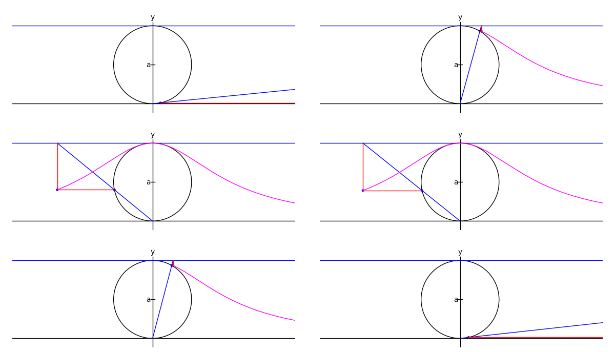
The witch of Maria Agnesi

by Marshall Hampton
xtreme = 4.1
myaxes = line([[-xtreme,0],[xtreme,0]],rgbcolor = (0,0,0))
myaxes = myaxes + line([[0,-1],[0,2.1]],rgbcolor = (0,0,0))
a = 1.0
t = var('t')
npi = RDF(pi)
def agnesi(theta):
    mac = circle((0,a),a,rgbcolor = (0,0,0))
    maL = line([[-xtreme,2*a],[xtreme,2*a]])
    maL2 = line([[0,0],[2*a*cot(theta),2*a]])
    p1 = [2*a*cot(theta),2*a*sin(theta)^2]
    p2 = [2*a*cot(theta)-cot(theta)*(2*a-2*a*sin(theta)^2),2*a*sin(theta)^2]
    maL3 = line([p2,p1,[2*a*cot(theta),2*a]], rgbcolor = (1,0,0))
    map1 = point(p1)
    map2 = point(p2)
    am = line([[-.05,a],[.05,a]], rgbcolor = (0,0,0))
    at = text('a',[-.1,a], rgbcolor = (0,0,0))
    yt = text('y',[0,2.2], rgbcolor = (0,0,0))
    xt = text('x',[xtreme + .1,-.1], rgbcolor = (0,0,0))
    matext = at+yt+xt
    ma = mac+myaxes+maL+am+matext+maL2+map1+maL3+map2
    return ma

def witchy(theta):
    ma = agnesi(theta)
    agplot = parametric_plot([2*a*cot(t),2*a*sin(t)^2],[t,.001,theta], rgbcolor = (1,0,1))
    return ma+agplot

a2 = animate([witchy(i) for i in srange(.1,npi-.1,npi/60)]+[witchy(i) for i in srange(npi-.1,.1,-npi/60)], xmin = -3, xmax = 3, ymin = 0, ymax = 2.3, figsize = [6,2.3], axes = False)

a2.show()
A simpler hypotrochoid
The following animates a hypotrochoid
import operator

# The colors for various elements of the plot:
class color:
    stylus = (1, 0, 0)
    outer  = (.8, .8, .8)
    inner  = (0, 0, 1)
    plot   = (0, 0, 0)
    center = (0, 0, 0)
    tip    = (1, 0, 0)
# and the corresponding line weights:
class weight:
    stylus = 1
    outer  = 1
    inner  = 1
    plot   = 1
    center = 5
    tip    = 5

scale = 1            # The scale of the image
animation_delay = .1 # The delay between frames, in seconds

# Starting and ending t values
t_i = 0
t_f = 2*pi
# The t values of the animation frames
tvals = srange(t_i, t_f, (t_f-t_i)/60)

r_o = 8 # Outer circle radius
r_i = 2 # Inner circle radius
r_s = 3 # Stylus radius

# Coordinates of the center of the inner circle
x_c = lambda t: (r_o - r_i)*cos(t)
y_c = lambda t: (r_o - r_i)*sin(t)

# Parametric coordinates for the plot
x = lambda t: x_c(t) + r_s*cos(t*(r_o/r_i))
y = lambda t: y_c(t) - r_s*sin(t*(r_o/r_i))

# Maximum x and y values of the plot
x_max = r_o - r_i + r_s
y_max = find_maximum_on_interval(y, t_i, t_f)[0]

# The plots of the individual elements. Order is important; plots
# are stacked from bottom to top as they appear.
elements = (
    # The outer circle
    lambda t_f: circle((0, 0),               r_o, rgbcolor=color.outer, thickness=weight.outer),
    # The plot itself
    lambda t_f: parametric_plot((x, y), t_i, t_f, rgbcolor=color.plot,  thickness=weight.plot),
    # The inner circle
    lambda t_f: circle((x_c(t_f), y_c(t_f)), r_i, rgbcolor=color.inner, thickness=weight.inner),
    # The inner circle's center
    lambda t_f: point((x_c(t_f), y_c(t_f)),       rgbcolor=color.center,pointsize=weight.center),
    # The stylus
    lambda t_f: line([(x_c(t_f), y_c(t_f)), (x(t_f), y(t_f))], rgbcolor=color.stylus, thickness=weight.stylus),
    # The stylus' tip
    lambda t_f: point((x_c(t_f), y_c(t_f)),       rgbcolor=color.tip,   pointsize=weight.tip),
)

# Create the plots and animate them. The animate function renders an
# animated gif from the frames provided as its first argument.
# Though avid python programmers will find the syntax clear, an
# explanation is provided for novices.
animation = animate([sum(f(t) for f in elements)
                     for t in tvals],
                    xmin=-x_max, xmax=x_max,
                    ymin=-y_max, ymax=y_max,
                    figsize=(x_max*scale, y_max*scale * y_max/x_max))

animation.show(delay=animation_delay)

# The previous could be expressed more pedagogically as follows:
#
#   Evaluate each function in the elements array for the provided t
#   value:
#
#     plots = lambda t: f(t) for f in elements
#
#   Join a group of plots together to form a single plot:
#
#     def join_plots(plots):
#         result = plots[0]
#         for plot in plots[1:]:
#             result += plot
#         return result
#
#   or
#
#     join_plots = sum
#
#   Create an array of plots, one for each provided t value:
#
#     frames = [join_plots(plots(t)) for t in tvals]
#
#   Finally, animate the frames:
#
#     animation = animate(frames)
The Towers of Hanoi

by Pablo Angulo
def plot_towers(towers):
    '''Returns a plot of the towers of Hanoi

    Uses matrix_plot
    '''
    K=max(max(l) for l in towers if l)+1
    M=matrix(ZZ,K,6*K+7)
    #first tower
    for t in range(len(towers[0])):
        j = t
        k=towers[0][t]-1
        for l in range(K+1-k,K+2+k):
            M[K-1-j,l]=1
    #second tower
    for t in range(len(towers[1])):
        j = t
        k=towers[1][t]-1
        for l in range(3*K+3-k,3*K+4+k):
            M[K-1-j,l]=1
    #third tower
    for t in range(len(towers[2])):
        j = t
        k=towers[2][t]-1
        for l in range(5*K+5-k,5*K+6+k):
            M[K-1-j,l]=1

    return matrix_plot(M, axes=False)

def animate_towers(towers,a=0,b=1,c=2,k=-1):
    '''Move last k discs from column a into column b

    Assumes that the last k discs of column a are all smaller
    than the discs in columns b and c
    '''
    if k==0:  return
    if k==-1: k=len(towers[a])
    for t in animate_towers(towers,a,c,b,k-1):
        yield t
    disc = towers[a].pop()
    towers[b].append(disc)
    yield plot_towers(towers)
    for t in animate_towers(towers,c,b,a,k-1):
        yield t

towers = (range(4,0,-1),[],[])
initial = plot_towers(towers)
frame_list=[initial]+list(animate_towers(towers))
animate(frame_list, axes=False).show(delay=80)
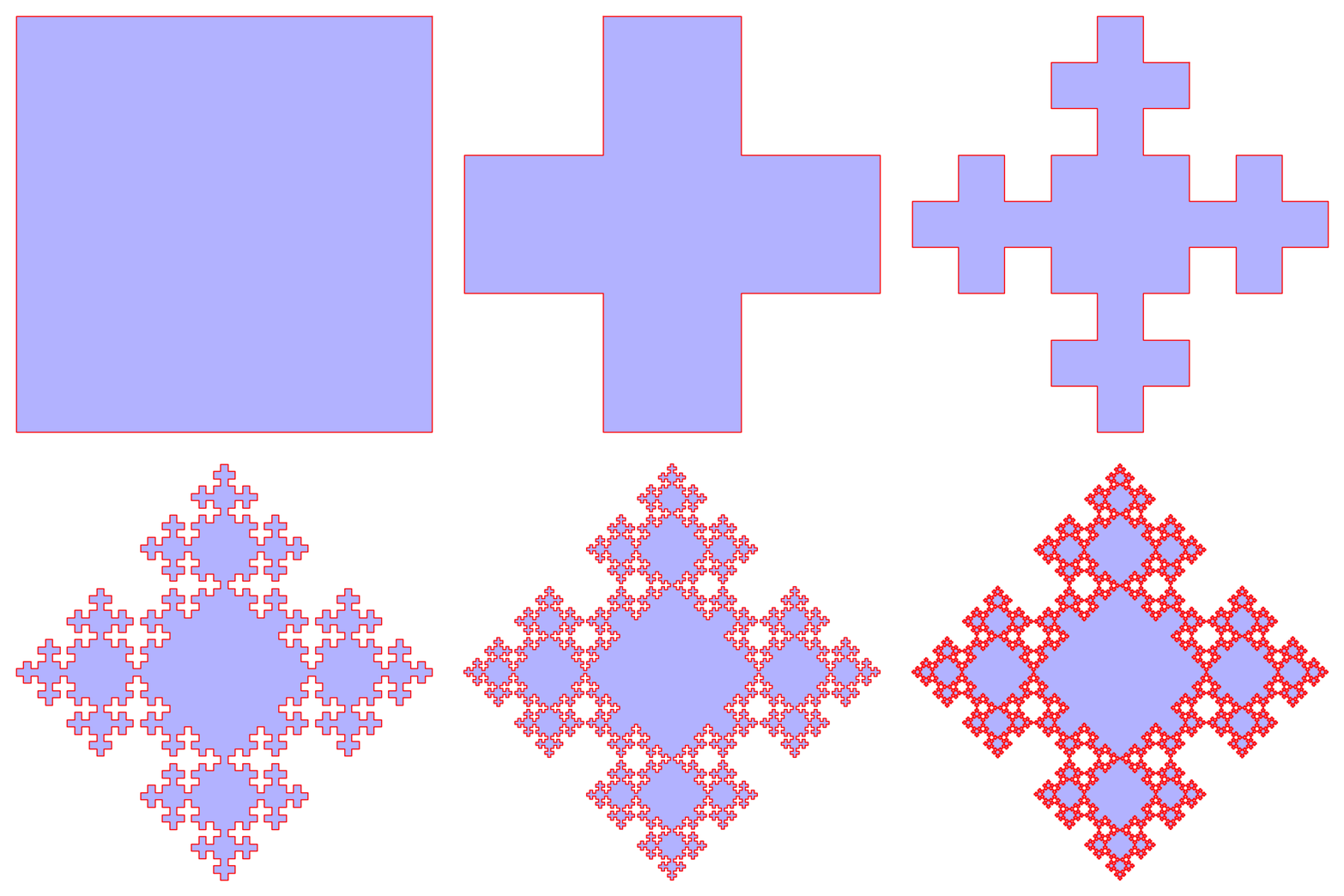
Fibonacci Tiles

by Sébastien Labbé
sage: path_op = dict(rgbcolor='red', thickness=1)
sage: fill_op = dict(rgbcolor='blue', alpha=0.3)
sage: options = dict(pathoptions=path_op, filloptions=fill_op, endarrow=False, startpoint=False)
sage: G = [words.fibonacci_tile(i).plot(**options) for i in range(7)]
sage: a = animate(G)
sage: a.show(delay=150)
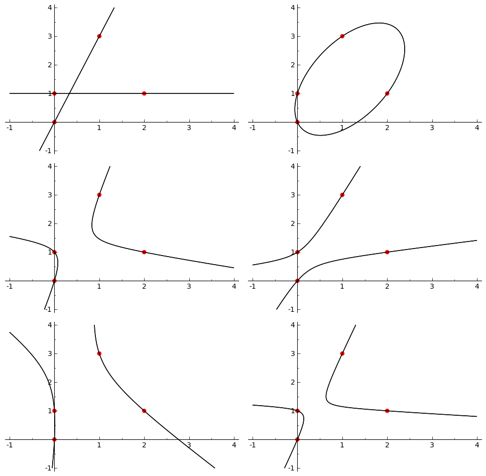
Pencil of conics
by Pablo Angulo 
puntos = [(0,0),(0,1),(1,3),(2,1)]
K = len(puntos)

var('x y')
coefs = matrix(QQ, K, 6)
for j in range(K):
    x0, y0 = puntos[j]
    coefs[j,:] = vector([x0^2, y0^2, x0*y0, x0, y0, 1])

K = coefs.right_kernel()
v1 = K.basis()[0]
v2 = K.basis()[1]

graficas = []
for t in srange(0,2*pi,0.3):
    c1, c2 = sin(t), cos(t)
    a,b,c,d,e,f = c1*v1 + c2*v2
    curva = a*x^2 + b*y^2 + c*x*y + d*x + e*y + f
    graficas.append( point2d(puntos,color=(1,0,0),pointsize=30) +
                     implicit_plot(curva,(x,-1,4),(y,-1,4)) )
a = animate(graficas)

a.show(delay=10)