|
Size: 1534
Comment:
|
← Revision 68 as of 2022-01-21 22:05:40 ⇥
Size: 24133
Comment:
|
| Deletions are marked like this. | Additions are marked like this. |
| Line 1: | Line 1: |
| = Sage-related art = * [http://sage.math.washington.edu/home/malb/graphics/banner/sagelogo.png logo] * [http://modular.math.washington.edu/sage/days2/sage-car.png Sage car] * [attachment:BadMugDesign.jpg Mug design, too dark though] == Sage Days 2 == * [http://sage.math.washington.edu/home/wdj/art/poster-sagedays1.jpg poster 1] (jpg) * [http://sage.math.washington.edu/home/wdj/art/poster-sagedays2.jpg poster 2] (jpg) * [http://sage.math.washington.edu/home/wdj/art/poster-sagedays3.jpg poster 3] (jpg) A flyer: * [http://sage.math.washington.edu/home/wdj/art/sagedays2flyer.pdf flyer] (pdf) A mosaic: * [http://sage.math.washington.edu/home/wdj/art/sagedays2mosaic.jpg mosaic] (jpg) * [http://sage.math.washington.edu/home/wdj/art/sage-motivational-poster.jpg poster 1] (jpg) * [http://sage.math.washington.edu/home/wdj/art/sage-motivational-poster2.jpg poster 2] (jpg) == Sage Days 3 == * [http://modular.math.washington.edu/home/wdj/art/sd3-motivator-mozaic.jpg mosaic poster] * [http://modular.math.washington.edu/home/wdj/art/sd3-motivator-poster.jpg poster with SAGE graphic] * [http://modular.math.washington.edu/home/wdj/art/sd3-magazine-cover.jpg magazine-cover style poster] * [http://sage.math.washington.edu/home/boothby/icons/sagedays3.1.png sage days 3 logo] == Sage Days 4 == * [http://www.sagemath.org/flier/flier.pdf Poster] == Joint meetings 2008 == * [http://sage.math.washington.edu/home/malb/graphics/banner.png Banner idea (not used)] |
This page contains animations and pictures drawn using [[https://www.sagemath.org|Sage]]. One can create an animation (.gif) in Sage from a list of graphics objects using the {{{animate}}} command. Currently, to export an animation in .gif format, you might need to install the [[https://www.imagemagick.org|ImageMagick]] command line tools package (the ``convert`` command). See the documentation for more information: {{{ sage: animate? }}} <<TableOfContents>> = Animations = == The witch of Maria Agnesi == {{attachment:witch.gif}} by Marshall Hampton {{{#!python numbers=none xtreme = 4.1 myaxes = line([[-xtreme,0],[xtreme,0]],rgbcolor = (0,0,0)) myaxes = myaxes + line([[0,-1],[0,2.1]],rgbcolor = (0,0,0)) a = 1.0 t = var('t') npi = RDF(pi) def agnesi(theta): mac = circle((0,a),a,rgbcolor = (0,0,0)) maL = line([[-xtreme,2*a],[xtreme,2*a]]) maL2 = line([[0,0],[2*a*cot(theta),2*a]]) p1 = [2*a*cot(theta),2*a*sin(theta)^2] p2 = [2*a*cot(theta)-cot(theta)*(2*a-2*a*sin(theta)^2),2*a*sin(theta)^2] maL3 = line([p2,p1,[2*a*cot(theta),2*a]], rgbcolor = (1,0,0)) map1 = point(p1) map2 = point(p2) am = line([[-.05,a],[.05,a]], rgbcolor = (0,0,0)) at = text('a',[-.1,a], rgbcolor = (0,0,0)) yt = text('y',[0,2.2], rgbcolor = (0,0,0)) xt = text('x',[xtreme + .1,-.1], rgbcolor = (0,0,0)) matext = at+yt+xt ma = mac+myaxes+maL+am+matext+maL2+map1+maL3+map2 return ma def witchy(theta): ma = agnesi(theta) agplot = parametric_plot([2*a*cot(t),2*a*sin(t)^2],[t,.001,theta], rgbcolor = (1,0,1)) return ma+agplot a2 = animate([witchy(i) for i in srange(.1,npi-.1,npi/60)]+[witchy(i) for i in srange(npi-.1,.1,-npi/60)], xmin = -3, xmax = 3, ymin = 0, ymax = 2.3, figsize = [6,2.3], axes = False) a2.show() }}} === A simpler hypotrochoid === The following animates a hypotrochoid {{{#!python numbers=off import operator # The colors for various elements of the plot: class color: stylus = (1, 0, 0) outer = (.8, .8, .8) inner = (0, 0, 1) plot = (0, 0, 0) center = (0, 0, 0) tip = (1, 0, 0) # and the corresponding line weights: class weight: stylus = 1 outer = 1 inner = 1 plot = 1 center = 5 tip = 5 scale = 1 # The scale of the image animation_delay = .1 # The delay between frames, in seconds # Starting and ending t values t_i = 0 t_f = 2*pi # The t values of the animation frames tvals = srange(t_i, t_f, (t_f-t_i)/60) r_o = 8 # Outer circle radius r_i = 2 # Inner circle radius r_s = 3 # Stylus radius # Coordinates of the center of the inner circle x_c = lambda t: (r_o - r_i)*cos(t) y_c = lambda t: (r_o - r_i)*sin(t) # Parametric coordinates for the plot x = lambda t: x_c(t) + r_s*cos(t*(r_o/r_i)) y = lambda t: y_c(t) - r_s*sin(t*(r_o/r_i)) # Maximum x and y values of the plot x_max = r_o - r_i + r_s y_max = find_maximum_on_interval(y, t_i, t_f)[0] # The plots of the individual elements. Order is important; plots # are stacked from bottom to top as they appear. elements = ( # The outer circle lambda t_f: circle((0, 0), r_o, rgbcolor=color.outer, thickness=weight.outer), # The plot itself lambda t_f: parametric_plot((x, y), t_i, t_f, rgbcolor=color.plot, thickness=weight.plot), # The inner circle lambda t_f: circle((x_c(t_f), y_c(t_f)), r_i, rgbcolor=color.inner, thickness=weight.inner), # The inner circle's center lambda t_f: point((x_c(t_f), y_c(t_f)), rgbcolor=color.center,pointsize=weight.center), # The stylus lambda t_f: line([(x_c(t_f), y_c(t_f)), (x(t_f), y(t_f))], rgbcolor=color.stylus, thickness=weight.stylus), # The stylus' tip lambda t_f: point((x_c(t_f), y_c(t_f)), rgbcolor=color.tip, pointsize=weight.tip), ) # Create the plots and animate them. The animate function renders an # animated gif from the frames provided as its first argument. # Though avid python programmers will find the syntax clear, an # explanation is provided for novices. animation = animate([sum(f(t) for f in elements) for t in tvals], xmin=-x_max, xmax=x_max, ymin=-y_max, ymax=y_max, figsize=(x_max*scale, y_max*scale * y_max/x_max)) animation.show(delay=animation_delay) # The previous could be expressed more pedagogically as follows: # # Evaluate each function in the elements array for the provided t # value: # # plots = lambda t: f(t) for f in elements # # Join a group of plots together to form a single plot: # # def join_plots(plots): # result = plots[0] # for plot in plots[1:]: # result += plot # return result # # or # # join_plots = sum # # Create an array of plots, one for each provided t value: # # frames = [join_plots(plots(t)) for t in tvals] # # Finally, animate the frames: # # animation = animate(frames) }}} == The Towers of Hanoi == {{attachment:hanoi.gif}} by Pablo Angulo {{{#!python numbers=off def plot_towers(towers): """ Return a plot of the towers of Hanoi. This uses matrix_plot. """ K = max(max(l) for l in towers if l) + 1 M = matrix(ZZ, K, 6 * K + 7) # first tower for t in range(len(towers[0])): j = t k = towers[0][t] - 1 for l in range(K+1-k,K+2+k): M[K-1-j,l] = 1 # second tower for t in range(len(towers[1])): j = t k = towers[1][t] - 1 for l in range(3*K+3-k,3*K+4+k): M[K-1-j,l] = 1 # third tower for t in range(len(towers[2])): j = t k = towers[2][t]-1 for l in range(5*K+5-k,5*K+6+k): M[K-1-j,l] = 1 return matrix_plot(M, axes=False) def animate_towers(towers,a=0,b=1,c=2,k=-1): '''Move last k discs from column a into column b Assumes that the last k discs of column a are all smaller than the discs in columns b and c ''' if k==0: return if k==-1: k=len(towers[a]) for t in animate_towers(towers,a,c,b,k-1): yield t disc = towers[a].pop() towers[b].append(disc) yield plot_towers(towers) for t in animate_towers(towers,c,b,a,k-1): yield t towers = (range(4,0,-1),[],[]) initial = plot_towers(towers) frame_list=[initial]+list(animate_towers(towers)) animate(frame_list, axes=False).show(delay=80) }}} == Fibonacci Tiles == {{attachment:fibotile.gif}} by Sébastien Labbé {{{#!python numbers=off sage: path_op = dict(rgbcolor='red', thickness=1) sage: fill_op = dict(rgbcolor='blue', alpha=0.3) sage: options = dict(pathoptions=path_op, filloptions=fill_op, endarrow=False, startpoint=False) sage: G = [words.fibonacci_tile(i).plot(**options) for i in range(7)] sage: a = animate(G) sage: a.show(delay=150) }}} == Pencil of conics == by Pablo Angulo {{attachment:pencil.gif}} {{{ puntos = [(0,0),(0,1),(1,3),(2,1)] K = len(puntos) var('x y') coefs = matrix(QQ, K, 6) for j in range(K): x0, y0 = puntos[j] coefs[j,:] = vector([x0^2, y0^2, x0*y0, x0, y0, 1]) K = coefs.right_kernel() v1 = K.basis()[0] v2 = K.basis()[1] graficas = [] for t in srange(0,2*pi,0.3): c1, c2 = sin(t), cos(t) a,b,c,d,e,f = c1*v1 + c2*v2 curva = a*x^2 + b*y^2 + c*x*y + d*x + e*y + f graficas.append( point2d(puntos,color=(1,0,0),pointsize=30) + implicit_plot(curva,(x,-1,4),(y,-1,4)) ) a = animate(graficas) a.show(delay=10) }}} = Pictures = These pictures and images were drawn by [[https://www.sagemath.org|Sage]]. == Snowman == * Fun art of spheres and cones: {{{#!python numbers=none from sage.plot.plot3d.shapes import Cone, Sphere r_bot = 3 r_mid = 2.25 r_top = 1.75 z_bot = r_bot z_mid = z_bot + r_bot + 1/2 * r_mid z_top = z_mid + r_mid + 1/2 * r_top # scale factors to shrink spheres along one axis s_body = 3/4 # vertical scale for body s_btns = 1/4 # horizontal scale for buttons s_eyes = 3/4 # horizontal scale for eyes z_bot_s = s_body * z_bot z_mid_s = s_body * z_mid z_top_s = s_body * z_top nose_length = 3/2*r_top r_button = 1/4 r_nose = 1/4 r_eye = 1/8 body_color = 'white' button_color = 'red' eye_color = 'black' nose_color = 'orange' body_bot = sphere((0, 0, z_bot), r_bot, color=body_color) body_mid = sphere((0, 0, z_mid), r_mid, color=body_color) body_top = sphere((0, 0, z_top), r_top, color=body_color) body = (body_bot + body_mid + body_top).scale(1, 1, s_body) button = Sphere(r_button, color=button_color).scale(s_btns, 1, 1) button_bot = button.translate(r_bot, 0, z_bot_s) button_mid = button.translate(r_mid, 0, z_mid_s) buttons = button_bot + button_mid eye_angle = pi/10 eye = Sphere(r_eye, color=eye_color).scale(s_eyes, 1, 1) eye = eye.translate((r_top, 0, z_top_s)) eyes = sum(eye.rotateZ(t) for t in (-eye_angle, eye_angle)) nose = Cone(r_nose, nose_length, color=nose_color) nose = nose.rotateY(-9/8*pi/2).translate(0, 0, z_top_s) parts = [body, buttons, eyes, nose] snowie = sum(parts) snowie.show(frame=False) }}} [[attachment:snowman.png|{{attachment:snowman.png||width=400}}]] == Everywhere continuous, nowhere differentiable function == * Everywhere continuous, nowhere differentiable function (in the infinite limit, anyway): {{{#!python numbers=none p = Graphics() for n in range(1,20): f = lambda x: sum([sin(x*3^i)/(2^i) for i in range(1,n)]) p += plot(f,0,float(pi/3),plot_points=2000,rgbcolor=hue(n/20)) p.show(xmin=0, ymin=0,dpi=250) }}} [[attachment:Fourier_series_wiki.png|{{attachment:Fourier_series_wiki.png||width=400}}]] == Mirrored balls in tachyon == {{{#!python numbers=none t = Tachyon(camera_center=(8.5,5,5.5), look_at=(2,0,0), raydepth=6, xres=1500, yres=1500) t.light((10,3,4), 1, (1,1,1)) t.texture('mirror', ambient=0.05, diffuse=0.05, specular=.9, opacity=0.9, color=(.8,.8,.8)) t.texture('grey', color=(.8,.8,.8), texfunc=7) ## try other values of texfunc too! t.plane((0,0,0),(0,0,1),'grey') t.sphere((4,-1,1), 1, 'mirror') t.sphere((0,-1,1), 1, 'mirror') t.sphere((2,-1,1), 0.5, 'mirror') t.sphere((2,1,1), 0.5, 'mirror') show(t) }}} [[attachment:Spheres_tachyon_wiki.png|{{attachment:Spheres_tachyon_wiki.png||width=400}}]] == Math art by Tom Boothby == {{{#!python numbers=none # Author: Tom Boothby # This is a remake of an old art piece I made in POVRay t = Tachyon(xres=1000,yres=600, camera_center=(1,0,5), antialiasing=3) t.light((4,3,2), 0.2, (1,1,1)) t.texture('t0', ambient=0.1, diffuse=0.9, specular=0.5, opacity=1.0, color=(1.0,1,1)) t.texture('t1', ambient=0.5, diffuse=0.5, specular=0.0, opacity=1.0, color=(0,0,0)) t.texture('t2', ambient=0.2, diffuse=0.7, specular=0, opacity=0.7, color=(.5,.5,.5)) t.texture('t3', ambient=.9, diffuse=5, specular=0,opacity=.1, color=(1,0,0)) t.sphere((1,0,0), 30, 't2') k=0 for i in srange(-pi*10,0,.01): k += 1 t.sphere((cos(i/10)-.1, sin(i/10)*cos(i), sin(i/10)*sin(i)), 0.1, 't0') t.sphere((cos(i/10) + 2.1, sin(i/10)*cos(i), sin(i/10)*sin(i)), 0.1, 't1') t.show(verbose=1) }}} [[attachment:Spirals_tachyon_wiki.png|{{attachment:Spirals_tachyon_wiki.png||width=400}}]] == Twisted cubic in tachyon == {{{#!python numbers=none t = Tachyon(xres=512,yres=512, camera_center=(5,0,0)) t.light((4,3,2), 0.2, (1,1,1)) t.texture('t0', ambient=0.1, diffuse=0.9, specular=0.5, opacity=1.0, color=(1.0,0,0)) t.texture('t1', ambient=0.1, diffuse=0.9, specular=0.3, opacity=1.0, color=(0,1.0,0)) t.texture('t2', ambient=0.2, diffuse=0.7, specular=0.5, opacity=0.7, color=(0,0,1.0)) k=0 for i in srange(-5,1.5,0.1): k += 1 t.sphere((i,i^2-0.5,i^3), 0.1, 't%s'%(k%3)) t.show() }}} [[attachment:Twisted_cubic_tachyon_wiki.png|{{attachment:Twisted_cubic_tachyon_wiki.png||width=400}}]] == Reflections from four spheres in tachyon == {{{#!python numbers=none t6 = Tachyon(camera_center=(0,-4,1), xres = 800, yres = 600, raydepth = 12, aspectratio=.75, antialiasing = True) t6.light((0.02,0.012,0.001), 0.01, (1,0,0)) t6.light((0,0,10), 0.01, (0,0,1)) t6.texture('s', color = (.8,1,1), opacity = .9, specular = .95, diffuse = .3, ambient = 0.05) t6.texture('p', color = (0,0,1), opacity = 1, specular = .2) t6.sphere((-1,-.57735,-0.7071),1,'s') t6.sphere((1,-.57735,-0.7071),1,'s') t6.sphere((0,1.15465,-0.7071),1,'s') t6.sphere((0,0,0.9259),1,'s') t6.plane((0,0,-1.9259),(0,0,1),'p') t6.show() }}} [[attachment:Blue_fractal_tachyon_wiki.png|{{attachment:Blue_fractal_tachyon_wiki.png||width=400}}]] == A cone inside a sphere == {{{#!python numbers=none sage: u,v = var("u,v") sage: p1 = parametric_plot3d([cos(u)*v, sin(u)*v, 3*v/2-1/3], (u, 0, 2*pi), (v, 0, 0.95),plot_points=[20,20]) sage: p2 = sphere((0,0,2/3), color='red', opacity=0.5, aspect_ratio=[1,1,1]) sage: show(p1+p2) }}} {{http://sage.math.washington.edu/home/wdj/art/cone-inside-sphere.jpg}} == A cylinder inside a cone == {{{#!python numbers=none sage: u,v = var("u,v") sage: p1 = parametric_plot3d([cos(u)*v, sin(u)*v, 3/2-3*v/2], (u, 0, 2*pi), (v, 0, 1.5), opacity = 0.5, plot_points=[20,20]) sage: p2 = parametric_plot3d([cos(u)/2, sin(u)/2, v-3/4], (u, 0, 2*pi), (v, 0, 3/2), plot_points=[20,20]) sage: show(p1+p2) }}} {{http://sage.math.washington.edu/home/wdj/art/cylinder-inside-cone.jpg}} == p-adic Seasons Greetings == * I know this is early, but thanks to Robert Bradshaw's p-adic plot function, here is a p-adic Seasons Greetings: [[attachment:Blue_fractal_tachyon_wiki.png|{{attachment:Greetings_wiki.png||width=400}}]] Here is the code: {{{#!python numbers=none sage: P1 = Zp(3).plot(rgbcolor=(0,1,0)) sage: P2 = Zp(7).plot(rgbcolor=(1,0,0)) sage: P3 = text("$Seasons$ $Greetings$ ",(0.0,1.8)) sage: P4 = text("$from$ $everyone$ $at$ sagemath.org!",(0.1,-1.6)) sage: (P1+P2+P3+P4).show(axes=False) }}} == Lorentz butterfly == {{{#!python numbers=off """ Draws Lorentz butterfly using matplotlib (2d) or jmol (3d). Written by Matthew Miller and William Stein. """ def butterfly2d(): """" EXAMPLES:: sage: butterfly2d() """ g = Graphics() x1, y1 = 0, 0 from math import sin, cos, exp, pi for theta in srange( 0, 10*pi, 0.01 ): r = exp(cos(theta)) - 2*cos(4*theta) + sin(theta/12)^5 x = r * cos(theta) # Convert polar to rectangular coordinates y = r * sin(theta) xx = x*6 + 25 # Scale factors to enlarge and center the curve. yy = y*6 + 25 if theta != 0: l = line( [(x1, y1), (xx, yy)], rgbcolor=hue(theta/7 + 4) ) g = g + l x1, y1 = xx, yy g.show(dpi=100, axes=False) def butterfly3d(): """" EXAMPLES:: sage: butterfly3d() """ g = point3d((0,0,0)) x1, y1 = 0, 0 from math import sin, cos, exp, pi for theta in srange( 0, 10*pi, 0.05): r = exp(cos(theta)) - 2*cos(4*theta) + sin(theta/12)^5 x = r * cos(theta) # Convert polar to rectangular coordinates y = r * sin(theta) xx = x*6 + 25 # Scale factors to enlarge and center the curve. yy = y*6 + 25 if theta != 0: l = line3d( [(x1, y1, theta), (xx, yy, theta)], rgbcolor=hue(theta/7 + 4) ) g = g + l x1, y1 = xx, yy g.show(dpi=100, axes=False) }}} [[attachment:Butterfly_2d_wiki.png|{{attachment:Butterfly_2d_wiki.png||width=400}}]] {{http://sage.math.washington.edu/home/wdj/art/butterfly3d.png}} == Feigenbaum diagram == Author: Pablo Angulo Posted to sage-devel 2008-09-13. See also https://sage.math.washington.edu:8101/home/pub/3 #Note: Mandelbrot set moved to interact/fractals {{{#!python numbers=off #Plots Feigenbaum diagram: divides the parameter interval [2,4] for mu #into N steps. For each value of the parameter, iterate the discrete #dynamical system x->mu*x*(1-x), drop the first M1 points in the orbit #and plot the next M2 points in a (mu,x) diagram N=200 M1=200 M2=200 x0=0.509434 puntos=[] for t in range(N): mu=2.0+2.0*t/N x=x0 for i in range(M1): x=mu*x*(1-x) for i in range(M2): x=mu*x*(1-x) puntos.append((mu,x)) point(puntos,pointsize=1) }}} [[attachment:feigenbaum.png|{{attachment:feigenbaum.png||width=400}}]] == Sierpinski triangle == * This was a black and white Sierpinski triangle coded by Marshall Hampton, with some slight tweeking by David Joyner to add colors: {{{#!python numbers=none def sierpinski_seasons_greetings(): """ Code by Marshall Hampton. Colors by David Joyner. General depth by Rob Beezer. Copyright Marshall Hampton 2008, licensed creative commons, attribution share-alike. """ depth = 7 nsq = RR(3^(1/2))/2.0 tlist_old = [[[-1/2.0,0.0],[1/2.0,0.0],[0.0,nsq]]] tlist_new = tlist_old[:] for ind in range(depth): for tri in tlist_old: for p in tri: new_tri = [[(p[0]+x[0])/2.0, (p[1]+x[1])/2.0] for x in tri] tlist_new.append(new_tri) tlist_old = tlist_new[:] T = tlist_old N = 4^depth N1 = N - 3^depth q1 = sum([line(T[i]+[T[i][0]], rgbcolor = (0,1,0)) for i in range(N1)]) q2 = sum([line(T[i]+[T[i][0]], rgbcolor = (1,0,0)) for i in range(N1,N)]) show(q2+q1, figsize = [6,6*nsq], axes = False) }}} [[attachment:Sierpinski_wiki.png|{{attachment:Sierpinski_wiki.png||width=400}}]] == Integral Curvature Apollonian Circle Packing == by Marshall Hampton and Carl Witty {{{ def kfun(k1,k2,k3,k4): """ The Descartes formula for the curvature of an inverted tangent circle. """ return 2*k1+2*k2+2*k3-k4 colorlist = [(1,0,1),(0,1,0),(0,0,1),(1,0,0)] def circfun(c1,c2,c3,c4): """ Computes the inversion of circle 4 in the first three circles. """ newk = kfun(c1[3],c2[3],c3[3],c4[3]) newx = (2*c1[0]*c1[3]+2*c2[0]*c2[3]+2*c3[0]*c3[3]-c4[0]*c4[3])/newk newy = (2*c1[1]*c1[3]+2*c2[1]*c2[3]+2*c3[1]*c3[3]-c4[1]*c4[3])/newk newcolor = c4[4] if newk > 0: newr = 1/newk elif newk < 0: newr = -1/newk else: newr = Infinity return [newx, newy, newr, newk, newcolor] def mcircle(circdata, label = False, thick = 1/10, cutoff = 2000, color = ''): """ Draws a circle from the data. label = True """ if color == '': color = colorlist[circdata[4]] if label==True and circdata[3] > 0 and circdata[2] > 1/cutoff: lab = text(str(circdata[3]),(circdata[0],circdata[1]), fontsize = \ 500*(circdata[2])^(.95), vertical_alignment = 'center', horizontal_alignment \ = 'center', rgbcolor = (0,0,0),zorder=10) else: lab = Graphics() circ = circle((circdata[0],circdata[1]), circdata[2], rgbcolor = (0,0,0), \ thickness = thick) circ = circ + circle((circdata[0],circdata[1]), circdata[2], rgbcolor = color, \ thickness = thick, fill=True, alpha = .4, zorder=0) return lab+circ def add_circs(c1, c2, c3, c4, cutoff = 300): """ Find the inversion of c4 through c1,c2,c3. Add the result to circlist, then (if the result is big enough) recurse. """ newcirc = circfun(c1, c2, c3, c4) if newcirc[3] < cutoff: circlist.append(newcirc) add_circs(newcirc, c1, c2, c3, cutoff = cutoff) add_circs(newcirc, c2, c3, c1, cutoff = cutoff) add_circs(newcirc, c3, c1, c2, cutoff = cutoff) zst1 = [0,0,1/2,-2,0] zst2 = [1/6,0,1/3,3,1] zst3 = [-1/3,0,1/6,6,2] zst4 = [-3/14,2/7,1/7,7,3] circlist = [zst1,zst2,zst3,zst4] add_circs(zst1,zst2,zst3,zst4,cutoff = 500) add_circs(zst2,zst3,zst4,zst1,cutoff = 500) add_circs(zst3,zst4,zst1,zst2,cutoff = 500) add_circs(zst4,zst1,zst2,zst3,cutoff = 500) circs = sum([mcircle(q, label = True, thick = 1/2) for q in \ circlist[1:]]) circs = circs + mcircle(circlist[0],color=(1,1,1),thick=1) circs.save('./Apollonian3.png',axes = False, figsize = [12,12], xmin = \ -1/2, xmax = 1/2, ymin = -1/2, ymax = 1/2) }}} [[attachment:Appolonian_wiki.png|{{attachment:Appolonian_wiki.png||width=400}}]] == Call graph of a recursive function == {{{ def grafo_llamadas(f): class G(object): def __init__(self, f): self.f=f self.stack = [] self.g = DiGraph() def __call__(self, *args): if self.stack: sargs = ','.join(str(a) for a in args) last = ','.join(str(a) for a in self.stack[-1]) if self.g.has_edge(last, sargs): l = self.g.edge_label(last, sargs) self.g.set_edge_label(last, sargs, l + 1) else: self.g.add_edge(last, sargs, 1) else: self.g = DiGraph() self.stack.append(args) v = self.f(*args) self.stack.pop() return v def grafo(self): return self.g return G(f) @grafo_llamadas def particiones(n, k): if k == n: return [[1]*n] if k == 1: return [[n]] if not(0 < k < n): return [] ls1 = [p+[1] for p in particiones(n-1, k-1)] ls2 = [[parte+1 for parte in p] for p in particiones(n-k, k)] return ls1 + ls2 particiones(13,5) g = particiones.grafo() g.show(edge_labels=True, figsize=(6,6), vertex_size=500, color_by_label=True) }}} [[attachment:Graph_call_wiki.png|{{attachment:Graph_call_wiki.png||width=400}}]] {{{ # D3js interactive version edge_partition = [ [edge for edge in g.edges() if edge[-1] == el] for el in set(g.edge_labels()) ] g.show(method='js', edge_labels=True, vertex_labels=True, link_distance=90, charge=-400, link_strength=2, force_spring_layout=True, edge_partition=edge_partition) }}} = Sage plotting = Here are some python plotting engines/libraries: Older/not python dedicated: * Grace: [[http://plasma-gate.weizmann.ac.il/Grace/|grace]], [[http://www.idyll.org/~n8gray/code|python interface]] * PGPLOT: [[http://efault.net/npat/hacks/ppgplot|ppgplot]], [[http://www.astro.caltech.edu/~tjp/pgplot/|pgplot]], [[http://astro.swarthmore.edu/~burns/pygplot/|pygplot]] * PLplot: http://www.plplot.org * opemath: Written by William Schelter and part of Maxima (thus also Sage) is a TCL/Tk plotting program which allows for interactive viewing. It has no separate download page. An example is this [[http://modular.math.washington.edu/home/wdj/art/saddle.png|saddle]]: {{{sage: maxima.eval("plot3d(2^(-u^2+v^2),[u,-1,1],[v,-1,1],[plot_format, openmath]);")}}} * Dislin: [[http://www.mps.mpg.de/dislin/|dislin]], [[http://kim.bio.upenn.edu/~pmagwene/disipyl.html|disipyl]] (a python wrapper for dislin). It's license says dislin is "free for non-commercial use". * Pyqwt at http://pyqwt.sourceforge.net/ is a plotting package requiring QT. It seems to have some 3d capabilities http://pyqwt.sourceforge.net/pyqwt3d-examples.html. Currently developed / good: * matplotlib: http://matplotlib.sourceforge.net * Tachyon: http://jedi.ks.uiuc.edu/~johns/raytracer/ Under active development: * Jmol: http://jmol.sourceforge.net/ Sage's plotting functionality is built on top of matplotlib, which is a very extensive plotting library with a user interface that is very similar to Matlab's plotting. The interface that Sage provides to matplotlib is very Mathematica like. There are also several links to plotting/graphics/data visualization programs at the scipy [[https://www.scipy.org/Topical_Software#head-b98ffdb309ccce4e4504a25ea75b5c806e4897b6|wiki]]. |
This page contains animations and pictures drawn using Sage. One can create an animation (.gif) in Sage from a list of graphics objects using the animate command. Currently, to export an animation in .gif format, you might need to install the ImageMagick command line tools package (the convert command). See the documentation for more information:
sage: animate?
Contents
- Animations
-
Pictures
- Snowman
- Everywhere continuous, nowhere differentiable function
- Mirrored balls in tachyon
- Math art by Tom Boothby
- Twisted cubic in tachyon
- Reflections from four spheres in tachyon
- A cone inside a sphere
- A cylinder inside a cone
- p-adic Seasons Greetings
- Lorentz butterfly
- Feigenbaum diagram
- Sierpinski triangle
- Integral Curvature Apollonian Circle Packing
- Call graph of a recursive function
- Sage plotting
Animations
The witch of Maria Agnesi
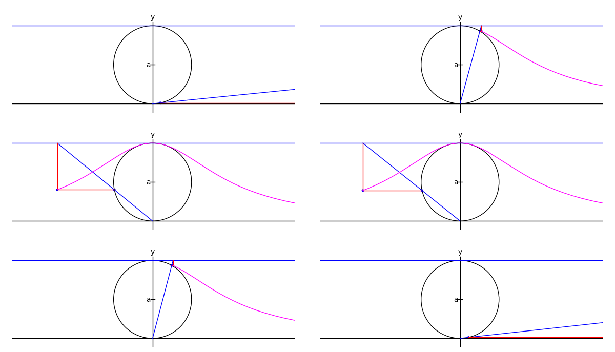
by Marshall Hampton
xtreme = 4.1
myaxes = line([[-xtreme,0],[xtreme,0]],rgbcolor = (0,0,0))
myaxes = myaxes + line([[0,-1],[0,2.1]],rgbcolor = (0,0,0))
a = 1.0
t = var('t')
npi = RDF(pi)
def agnesi(theta):
    mac = circle((0,a),a,rgbcolor = (0,0,0))
    maL = line([[-xtreme,2*a],[xtreme,2*a]])
    maL2 = line([[0,0],[2*a*cot(theta),2*a]])
    p1 = [2*a*cot(theta),2*a*sin(theta)^2]
    p2 = [2*a*cot(theta)-cot(theta)*(2*a-2*a*sin(theta)^2),2*a*sin(theta)^2]
    maL3 = line([p2,p1,[2*a*cot(theta),2*a]], rgbcolor = (1,0,0))
    map1 = point(p1)
    map2 = point(p2)
    am = line([[-.05,a],[.05,a]], rgbcolor = (0,0,0))
    at = text('a',[-.1,a], rgbcolor = (0,0,0))
    yt = text('y',[0,2.2], rgbcolor = (0,0,0))
    xt = text('x',[xtreme + .1,-.1], rgbcolor = (0,0,0))
    matext = at+yt+xt
    ma = mac+myaxes+maL+am+matext+maL2+map1+maL3+map2
    return ma

def witchy(theta):
    ma = agnesi(theta)
    agplot = parametric_plot([2*a*cot(t),2*a*sin(t)^2],[t,.001,theta], rgbcolor = (1,0,1))
    return ma+agplot

a2 = animate([witchy(i) for i in srange(.1,npi-.1,npi/60)]+[witchy(i) for i in srange(npi-.1,.1,-npi/60)], xmin = -3, xmax = 3, ymin = 0, ymax = 2.3, figsize = [6,2.3], axes = False)

a2.show()
A simpler hypotrochoid
The following animates a hypotrochoid
import operator

# The colors for various elements of the plot:
class color:
    stylus = (1, 0, 0)
    outer  = (.8, .8, .8)
    inner  = (0, 0, 1)
    plot   = (0, 0, 0)
    center = (0, 0, 0)
    tip    = (1, 0, 0)
# and the corresponding line weights:
class weight:
    stylus = 1
    outer  = 1
    inner  = 1
    plot   = 1
    center = 5
    tip    = 5

scale = 1            # The scale of the image
animation_delay = .1 # The delay between frames, in seconds

# Starting and ending t values
t_i = 0
t_f = 2*pi
# The t values of the animation frames
tvals = srange(t_i, t_f, (t_f-t_i)/60)

r_o = 8 # Outer circle radius
r_i = 2 # Inner circle radius
r_s = 3 # Stylus radius

# Coordinates of the center of the inner circle
x_c = lambda t: (r_o - r_i)*cos(t)
y_c = lambda t: (r_o - r_i)*sin(t)

# Parametric coordinates for the plot
x = lambda t: x_c(t) + r_s*cos(t*(r_o/r_i))
y = lambda t: y_c(t) - r_s*sin(t*(r_o/r_i))

# Maximum x and y values of the plot
x_max = r_o - r_i + r_s
y_max = find_maximum_on_interval(y, t_i, t_f)[0]

# The plots of the individual elements. Order is important; plots
# are stacked from bottom to top as they appear.
elements = (
    # The outer circle
    lambda t_f: circle((0, 0),               r_o, rgbcolor=color.outer, thickness=weight.outer),
    # The plot itself
    lambda t_f: parametric_plot((x, y), t_i, t_f, rgbcolor=color.plot,  thickness=weight.plot),
    # The inner circle
    lambda t_f: circle((x_c(t_f), y_c(t_f)), r_i, rgbcolor=color.inner, thickness=weight.inner),
    # The inner circle's center
    lambda t_f: point((x_c(t_f), y_c(t_f)),       rgbcolor=color.center,pointsize=weight.center),
    # The stylus
    lambda t_f: line([(x_c(t_f), y_c(t_f)), (x(t_f), y(t_f))], rgbcolor=color.stylus, thickness=weight.stylus),
    # The stylus' tip
    lambda t_f: point((x_c(t_f), y_c(t_f)),       rgbcolor=color.tip,   pointsize=weight.tip),
)

# Create the plots and animate them. The animate function renders an
# animated gif from the frames provided as its first argument.
# Though avid python programmers will find the syntax clear, an
# explanation is provided for novices.
animation = animate([sum(f(t) for f in elements)
                     for t in tvals],
                    xmin=-x_max, xmax=x_max,
                    ymin=-y_max, ymax=y_max,
                    figsize=(x_max*scale, y_max*scale * y_max/x_max))

animation.show(delay=animation_delay)

# The previous could be expressed more pedagogically as follows:
#
#   Evaluate each function in the elements array for the provided t
#   value:
#
#     plots = lambda t: f(t) for f in elements
#
#   Join a group of plots together to form a single plot:
#
#     def join_plots(plots):
#         result = plots[0]
#         for plot in plots[1:]:
#             result += plot
#         return result
#
#   or
#
#     join_plots = sum
#
#   Create an array of plots, one for each provided t value:
#
#     frames = [join_plots(plots(t)) for t in tvals]
#
#   Finally, animate the frames:
#
#     animation = animate(frames)
The Towers of Hanoi

by Pablo Angulo
def plot_towers(towers):
    """
    Return a plot of the towers of Hanoi.

    This uses matrix_plot.
    """
    K = max(max(l) for l in towers if l) + 1
    M = matrix(ZZ, K, 6 * K + 7)
    # first tower
    for t in range(len(towers[0])):
        j = t
        k = towers[0][t] - 1
        for l in range(K+1-k,K+2+k):
            M[K-1-j,l] = 1
    # second tower
    for t in range(len(towers[1])):
        j = t
        k = towers[1][t] - 1
        for l in range(3*K+3-k,3*K+4+k):
            M[K-1-j,l] = 1
    # third tower
    for t in range(len(towers[2])):
        j = t
        k = towers[2][t]-1
        for l in range(5*K+5-k,5*K+6+k):
            M[K-1-j,l] = 1

    return matrix_plot(M, axes=False)

def animate_towers(towers,a=0,b=1,c=2,k=-1):
    '''Move last k discs from column a into column b

    Assumes that the last k discs of column a are all smaller
    than the discs in columns b and c
    '''
    if k==0:  return
    if k==-1: k=len(towers[a])
    for t in animate_towers(towers,a,c,b,k-1):
        yield t
    disc = towers[a].pop()
    towers[b].append(disc)
    yield plot_towers(towers)
    for t in animate_towers(towers,c,b,a,k-1):
        yield t

towers = (range(4,0,-1),[],[])
initial = plot_towers(towers)
frame_list=[initial]+list(animate_towers(towers))
animate(frame_list, axes=False).show(delay=80)
Fibonacci Tiles
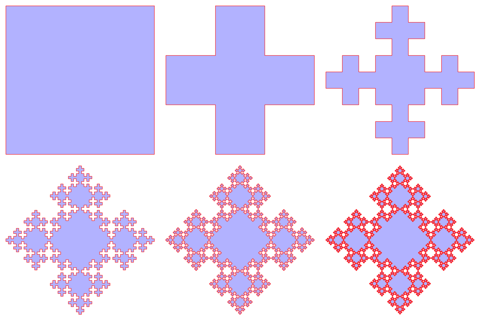
by Sébastien Labbé
sage: path_op = dict(rgbcolor='red', thickness=1)
sage: fill_op = dict(rgbcolor='blue', alpha=0.3)
sage: options = dict(pathoptions=path_op, filloptions=fill_op, endarrow=False, startpoint=False)
sage: G = [words.fibonacci_tile(i).plot(**options) for i in range(7)]
sage: a = animate(G)
sage: a.show(delay=150)
Pencil of conics
by Pablo Angulo 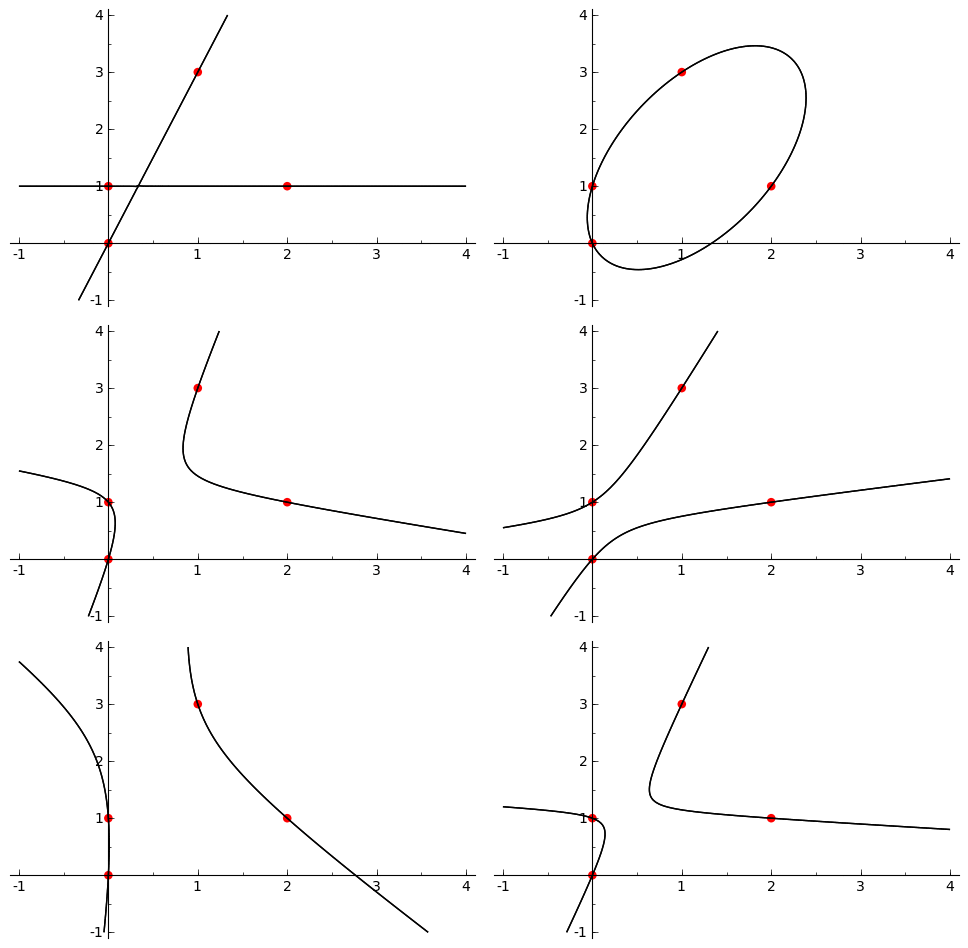
puntos = [(0,0),(0,1),(1,3),(2,1)]
K = len(puntos)

var('x y')
coefs = matrix(QQ, K, 6)
for j in range(K):
    x0, y0 = puntos[j]
    coefs[j,:] = vector([x0^2, y0^2, x0*y0, x0, y0, 1])

K = coefs.right_kernel()
v1 = K.basis()[0]
v2 = K.basis()[1]

graficas = []
for t in srange(0,2*pi,0.3):
    c1, c2 = sin(t), cos(t)
    a,b,c,d,e,f = c1*v1 + c2*v2
    curva = a*x^2 + b*y^2 + c*x*y + d*x + e*y + f
    graficas.append( point2d(puntos,color=(1,0,0),pointsize=30) +
                     implicit_plot(curva,(x,-1,4),(y,-1,4)) )
a = animate(graficas)

a.show(delay=10)
Pictures
These pictures and images were drawn by Sage.
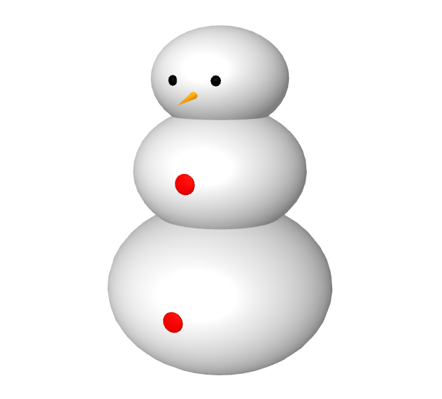
Snowman
- Fun art of spheres and cones:
from sage.plot.plot3d.shapes import Cone, Sphere

r_bot = 3
r_mid = 2.25
r_top = 1.75

z_bot = r_bot
z_mid = z_bot + r_bot + 1/2 * r_mid
z_top = z_mid + r_mid + 1/2 * r_top

# scale factors to shrink spheres along one axis

s_body = 3/4  # vertical scale for body
s_btns = 1/4  # horizontal scale for buttons
s_eyes = 3/4  # horizontal scale for eyes

z_bot_s = s_body * z_bot
z_mid_s = s_body * z_mid
z_top_s = s_body * z_top

nose_length = 3/2*r_top

r_button = 1/4
r_nose = 1/4
r_eye = 1/8

body_color = 'white'
button_color = 'red'
eye_color = 'black'
nose_color = 'orange'

body_bot = sphere((0, 0, z_bot), r_bot, color=body_color)
body_mid = sphere((0, 0, z_mid), r_mid, color=body_color)
body_top = sphere((0, 0, z_top), r_top, color=body_color)
body = (body_bot + body_mid + body_top).scale(1, 1, s_body)

button = Sphere(r_button, color=button_color).scale(s_btns, 1, 1)
button_bot = button.translate(r_bot, 0, z_bot_s)
button_mid = button.translate(r_mid, 0, z_mid_s)
buttons = button_bot + button_mid

eye_angle = pi/10
eye = Sphere(r_eye, color=eye_color).scale(s_eyes, 1, 1)
eye = eye.translate((r_top, 0, z_top_s))
eyes = sum(eye.rotateZ(t) for t in (-eye_angle, eye_angle))

nose = Cone(r_nose, nose_length, color=nose_color)
nose = nose.rotateY(-9/8*pi/2).translate(0, 0, z_top_s)

parts = [body, buttons, eyes, nose]
snowie = sum(parts)
snowie.show(frame=False)
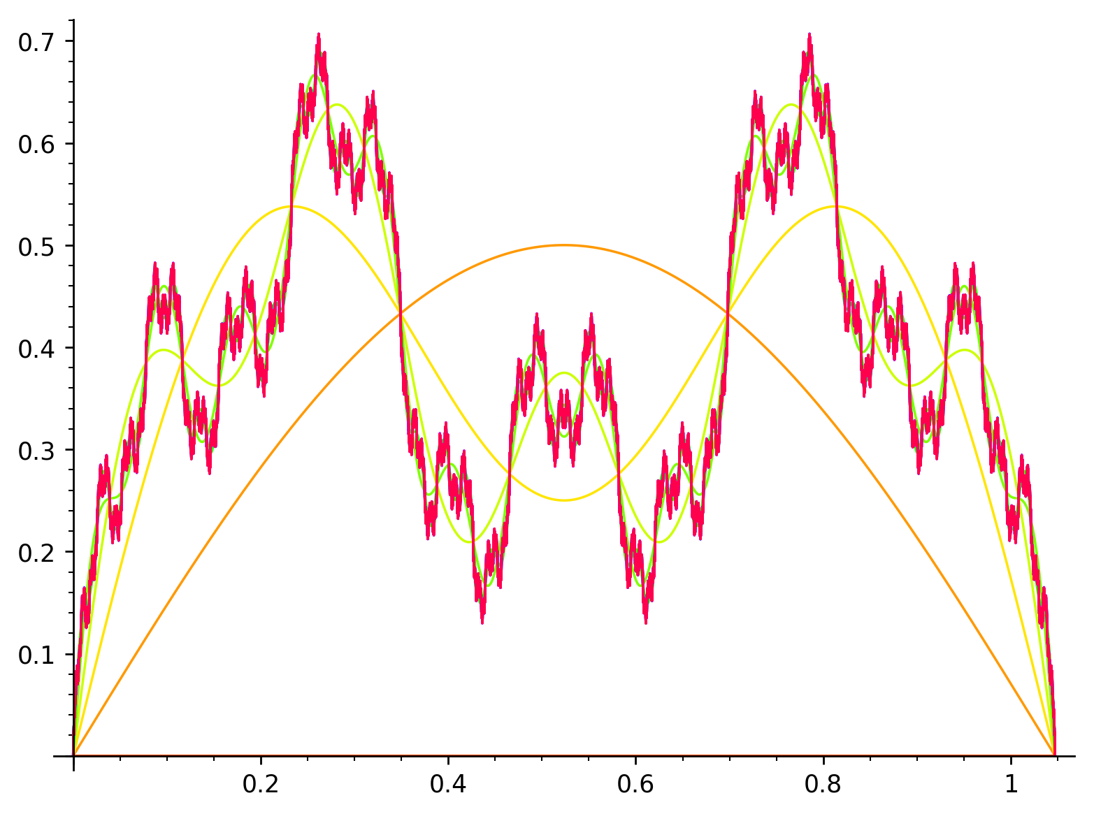
Everywhere continuous, nowhere differentiable function
- Everywhere continuous, nowhere differentiable function (in the infinite limit, anyway):
p = Graphics()
for n in range(1,20):
  f = lambda x: sum([sin(x*3^i)/(2^i) for i in range(1,n)])
  p += plot(f,0,float(pi/3),plot_points=2000,rgbcolor=hue(n/20))

p.show(xmin=0, ymin=0,dpi=250)
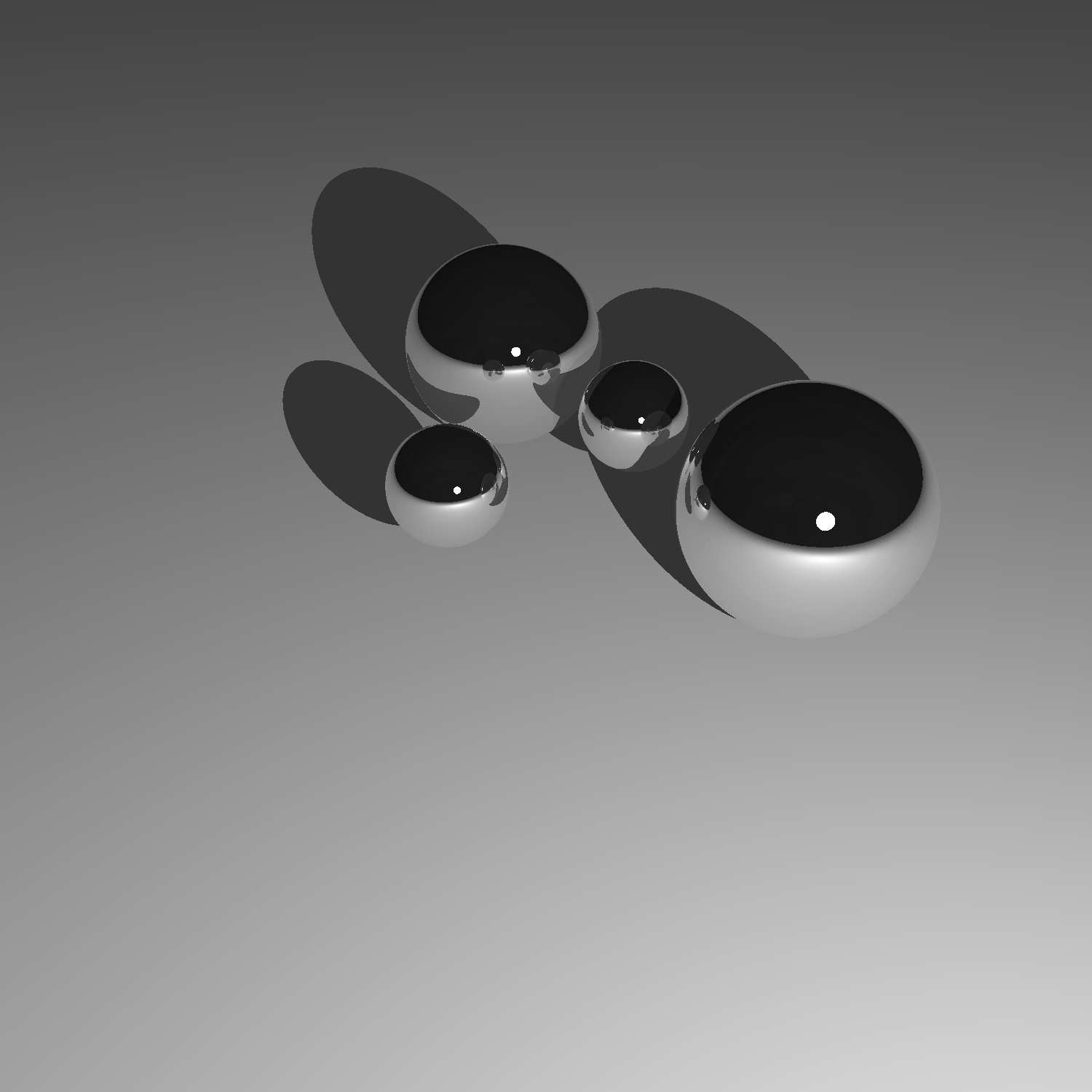
Mirrored balls in tachyon
t = Tachyon(camera_center=(8.5,5,5.5), look_at=(2,0,0), raydepth=6, xres=1500, yres=1500)
t.light((10,3,4), 1, (1,1,1))
t.texture('mirror', ambient=0.05, diffuse=0.05, specular=.9, opacity=0.9, color=(.8,.8,.8))
t.texture('grey', color=(.8,.8,.8), texfunc=7) ## try other values of texfunc too!
t.plane((0,0,0),(0,0,1),'grey')
t.sphere((4,-1,1), 1, 'mirror')
t.sphere((0,-1,1), 1, 'mirror')
t.sphere((2,-1,1), 0.5, 'mirror')
t.sphere((2,1,1), 0.5, 'mirror')
show(t)
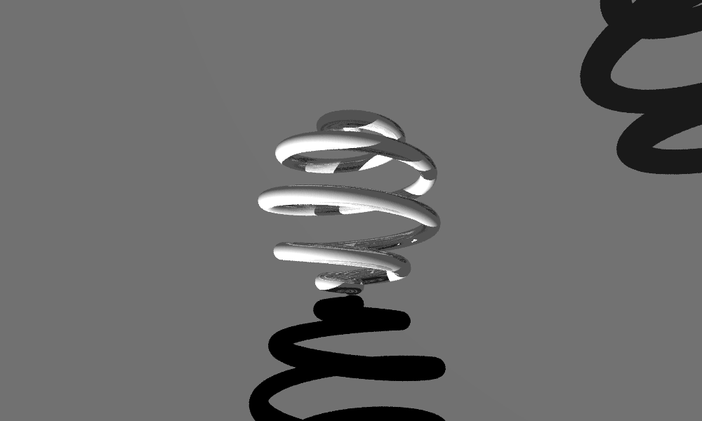
Math art by Tom Boothby
# Author: Tom Boothby
# This is a remake of an old art piece I made in POVRay


t = Tachyon(xres=1000,yres=600, camera_center=(1,0,5), antialiasing=3)
t.light((4,3,2), 0.2, (1,1,1))
t.texture('t0', ambient=0.1, diffuse=0.9, specular=0.5, opacity=1.0, color=(1.0,1,1))
t.texture('t1', ambient=0.5, diffuse=0.5, specular=0.0, opacity=1.0, color=(0,0,0))
t.texture('t2', ambient=0.2, diffuse=0.7, specular=0, opacity=0.7, color=(.5,.5,.5))
t.texture('t3', ambient=.9, diffuse=5, specular=0,opacity=.1, color=(1,0,0))
t.sphere((1,0,0), 30, 't2')


k=0
for i in srange(-pi*10,0,.01):
  k += 1
  t.sphere((cos(i/10)-.1, sin(i/10)*cos(i), sin(i/10)*sin(i)), 0.1, 't0')
  t.sphere((cos(i/10) + 2.1, sin(i/10)*cos(i), sin(i/10)*sin(i)), 0.1, 't1')

t.show(verbose=1)
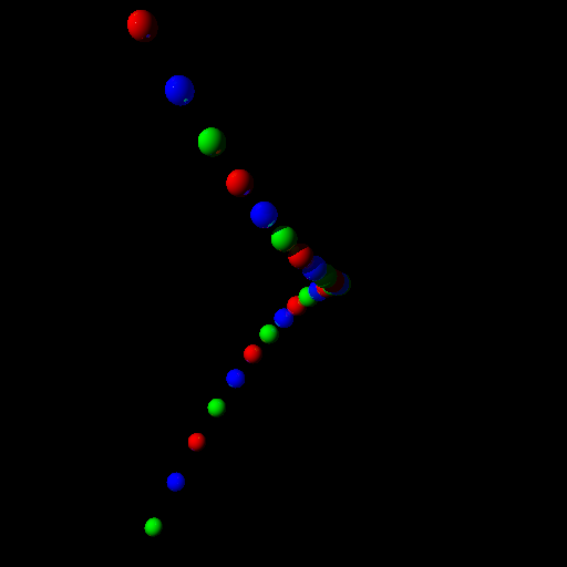
Twisted cubic in tachyon
t = Tachyon(xres=512,yres=512, camera_center=(5,0,0))
t.light((4,3,2), 0.2, (1,1,1))
t.texture('t0', ambient=0.1, diffuse=0.9, specular=0.5, opacity=1.0, color=(1.0,0,0))
t.texture('t1', ambient=0.1, diffuse=0.9, specular=0.3, opacity=1.0, color=(0,1.0,0))
t.texture('t2', ambient=0.2, diffuse=0.7, specular=0.5, opacity=0.7, color=(0,0,1.0))
k=0
for i in srange(-5,1.5,0.1):
    k += 1
    t.sphere((i,i^2-0.5,i^3), 0.1, 't%s'%(k%3))

t.show()
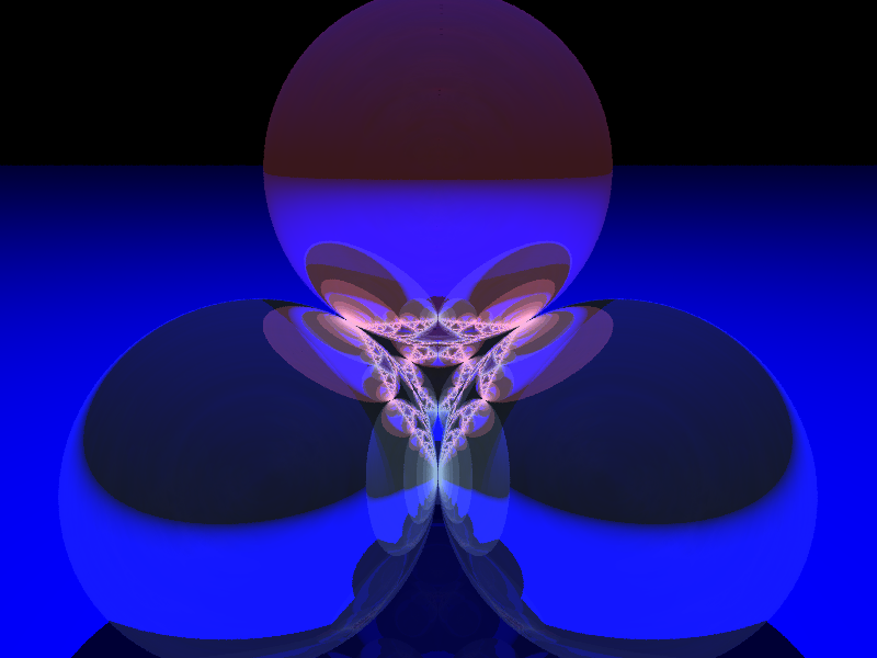
Reflections from four spheres in tachyon
t6 = Tachyon(camera_center=(0,-4,1), xres = 800, yres = 600, raydepth = 12, aspectratio=.75, antialiasing = True)
t6.light((0.02,0.012,0.001), 0.01, (1,0,0))
t6.light((0,0,10), 0.01, (0,0,1))
t6.texture('s', color = (.8,1,1), opacity = .9, specular = .95, diffuse = .3, ambient = 0.05)
t6.texture('p', color = (0,0,1), opacity = 1, specular = .2)
t6.sphere((-1,-.57735,-0.7071),1,'s')
t6.sphere((1,-.57735,-0.7071),1,'s')
t6.sphere((0,1.15465,-0.7071),1,'s')
t6.sphere((0,0,0.9259),1,'s')
t6.plane((0,0,-1.9259),(0,0,1),'p')
t6.show()
A cone inside a sphere
sage: u,v = var("u,v")
sage: p1 = parametric_plot3d([cos(u)*v, sin(u)*v, 3*v/2-1/3], (u, 0, 2*pi), (v, 0, 0.95),plot_points=[20,20])
sage: p2 = sphere((0,0,2/3), color='red', opacity=0.5, aspect_ratio=[1,1,1])
sage: show(p1+p2)

A cylinder inside a cone
sage: u,v = var("u,v")
sage: p1 = parametric_plot3d([cos(u)*v, sin(u)*v, 3/2-3*v/2], (u, 0, 2*pi), (v, 0, 1.5), opacity = 0.5, plot_points=[20,20])
sage: p2 = parametric_plot3d([cos(u)/2, sin(u)/2, v-3/4], (u, 0, 2*pi), (v, 0, 3/2), plot_points=[20,20])
sage: show(p1+p2)

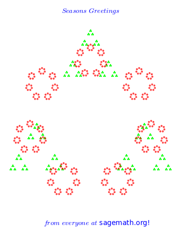
p-adic Seasons Greetings
- I know this is early, but thanks to Robert Bradshaw's p-adic plot function, here is a p-adic Seasons Greetings:
Here is the code:
sage: P1 = Zp(3).plot(rgbcolor=(0,1,0))
sage: P2 = Zp(7).plot(rgbcolor=(1,0,0))
sage: P3 = text("$Seasons$ $Greetings$ ",(0.0,1.8))
sage: P4 = text("$from$ $everyone$ $at$ sagemath.org!",(0.1,-1.6))
sage: (P1+P2+P3+P4).show(axes=False)
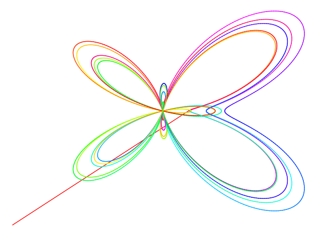
Lorentz butterfly
"""
Draws Lorentz butterfly using matplotlib (2d) or jmol (3d).
Written by Matthew Miller and William Stein.

"""

def butterfly2d():
    """"
    EXAMPLES::

        sage: butterfly2d()
    """
    g = Graphics()
    x1, y1 = 0, 0
    from math import sin, cos, exp, pi
    for theta in srange( 0, 10*pi, 0.01 ):
        r = exp(cos(theta)) - 2*cos(4*theta) + sin(theta/12)^5
        x = r * cos(theta)  # Convert polar to rectangular coordinates
        y = r * sin(theta)
        xx = x*6 + 25       # Scale factors to enlarge and center the curve.
        yy = y*6 + 25
        if theta != 0:
            l = line( [(x1, y1), (xx, yy)], rgbcolor=hue(theta/7 + 4) )
            g = g + l
            x1, y1 = xx, yy
    g.show(dpi=100, axes=False)

def butterfly3d():
    """"
    EXAMPLES::

        sage: butterfly3d()
    """
    g = point3d((0,0,0))
    x1, y1 = 0, 0
    from math import sin, cos, exp, pi
    for theta in srange( 0, 10*pi, 0.05):
        r = exp(cos(theta)) - 2*cos(4*theta) + sin(theta/12)^5
        x = r * cos(theta)  # Convert polar to rectangular coordinates
        y = r * sin(theta)
        xx = x*6 + 25       # Scale factors to enlarge and center the curve.
        yy = y*6 + 25
        if theta != 0:
            l = line3d( [(x1, y1, theta), (xx, yy, theta)],
            rgbcolor=hue(theta/7 + 4) )
            g = g + l
            x1, y1 = xx, yy
    g.show(dpi=100, axes=False)

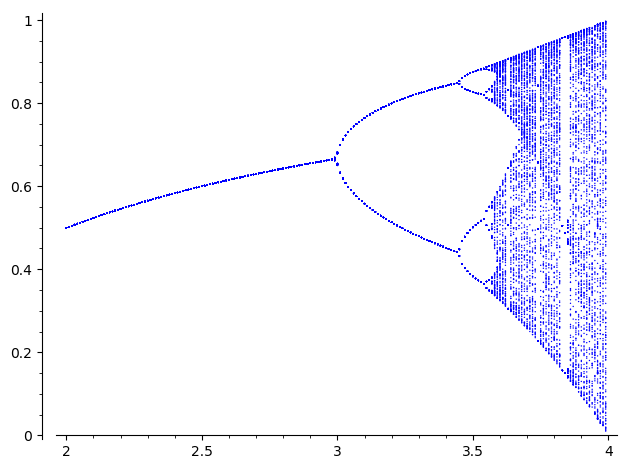
Feigenbaum diagram
Author: Pablo Angulo Posted to sage-devel 2008-09-13. See also https://sage.math.washington.edu:8101/home/pub/3 #Note: Mandelbrot set moved to interact/fractals
#Plots Feigenbaum diagram: divides the parameter interval [2,4] for mu
#into N steps. For each value of the parameter, iterate the discrete
#dynamical system x->mu*x*(1-x), drop the first M1 points in the orbit
#and plot the next M2 points in a (mu,x) diagram

N=200
M1=200
M2=200
x0=0.509434

puntos=[]
for t in range(N):
   mu=2.0+2.0*t/N
   x=x0
   for i in range(M1):
       x=mu*x*(1-x)
   for i in range(M2):
       x=mu*x*(1-x)
       puntos.append((mu,x))
point(puntos,pointsize=1)
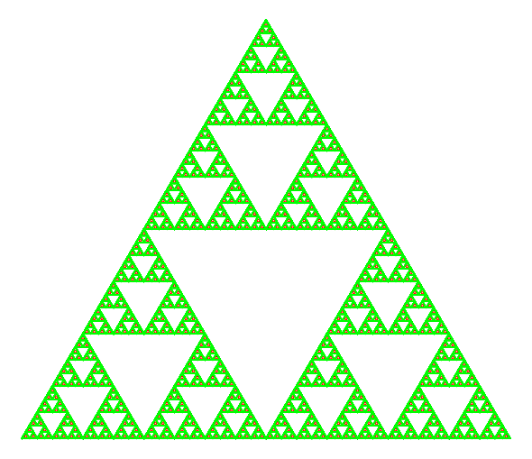
Sierpinski triangle
- This was a black and white Sierpinski triangle coded by Marshall Hampton, with some slight tweeking by David Joyner to add colors:
def sierpinski_seasons_greetings():
    """
    Code by Marshall Hampton.
    Colors by David Joyner.
    General depth by Rob Beezer.
    Copyright Marshall Hampton 2008, licensed
    creative commons, attribution share-alike.
    """
    depth = 7
    nsq = RR(3^(1/2))/2.0
    tlist_old = [[[-1/2.0,0.0],[1/2.0,0.0],[0.0,nsq]]]
    tlist_new = tlist_old[:]
    for ind in range(depth):
       for tri in tlist_old:
           for p in tri:
               new_tri = [[(p[0]+x[0])/2.0, (p[1]+x[1])/2.0] for x in tri]
               tlist_new.append(new_tri)
       tlist_old = tlist_new[:]
    T = tlist_old
    N  = 4^depth
    N1 = N - 3^depth
    q1 = sum([line(T[i]+[T[i][0]], rgbcolor = (0,1,0)) for i in range(N1)])
    q2 = sum([line(T[i]+[T[i][0]], rgbcolor = (1,0,0)) for i in range(N1,N)])
    show(q2+q1, figsize = [6,6*nsq], axes = False)
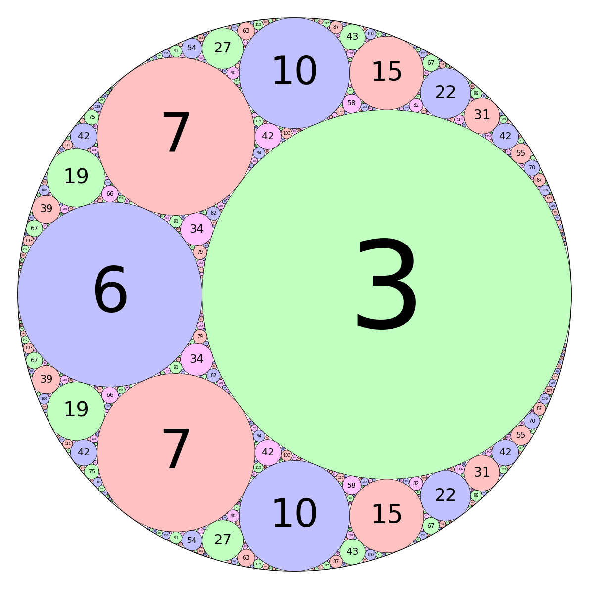
Integral Curvature Apollonian Circle Packing
by Marshall Hampton and Carl Witty
def kfun(k1,k2,k3,k4):
    """
    The Descartes formula for the curvature of an inverted tangent circle.
    """
    return 2*k1+2*k2+2*k3-k4


colorlist = [(1,0,1),(0,1,0),(0,0,1),(1,0,0)]

def circfun(c1,c2,c3,c4):
    """
    Computes the inversion of circle 4 in the first three circles.
    """
    newk = kfun(c1[3],c2[3],c3[3],c4[3])
    newx = (2*c1[0]*c1[3]+2*c2[0]*c2[3]+2*c3[0]*c3[3]-c4[0]*c4[3])/newk
    newy = (2*c1[1]*c1[3]+2*c2[1]*c2[3]+2*c3[1]*c3[3]-c4[1]*c4[3])/newk
    newcolor = c4[4]
    if newk > 0:
        newr = 1/newk
    elif newk < 0:
        newr = -1/newk
    else:
        newr = Infinity
    return [newx, newy, newr, newk, newcolor]

def mcircle(circdata, label = False, thick = 1/10, cutoff = 2000, color = ''):
    """
    Draws a circle from the data.  label = True
    """
    if color == '':
        color = colorlist[circdata[4]]
    if label==True and circdata[3] > 0 and circdata[2] > 1/cutoff:
        lab = text(str(circdata[3]),(circdata[0],circdata[1]), fontsize = \
500*(circdata[2])^(.95), vertical_alignment = 'center', horizontal_alignment \
= 'center', rgbcolor = (0,0,0),zorder=10)
    else:
        lab = Graphics()
    circ = circle((circdata[0],circdata[1]), circdata[2], rgbcolor = (0,0,0), \
thickness = thick)
    circ = circ + circle((circdata[0],circdata[1]), circdata[2], rgbcolor = color, \
thickness = thick, fill=True, alpha = .4, zorder=0)
    return lab+circ

def add_circs(c1, c2, c3, c4, cutoff = 300):
    """
    Find the inversion of c4 through c1,c2,c3.  Add the result to circlist,
    then (if the result is big enough) recurse.
    """
    newcirc = circfun(c1, c2, c3, c4)
    if newcirc[3] < cutoff:
        circlist.append(newcirc)
        add_circs(newcirc, c1, c2, c3, cutoff = cutoff)
        add_circs(newcirc, c2, c3, c1, cutoff = cutoff)
        add_circs(newcirc, c3, c1, c2, cutoff = cutoff)

zst1 = [0,0,1/2,-2,0]
zst2 = [1/6,0,1/3,3,1]
zst3 = [-1/3,0,1/6,6,2]
zst4 = [-3/14,2/7,1/7,7,3]

circlist = [zst1,zst2,zst3,zst4]
add_circs(zst1,zst2,zst3,zst4,cutoff = 500)
add_circs(zst2,zst3,zst4,zst1,cutoff = 500)
add_circs(zst3,zst4,zst1,zst2,cutoff = 500)
add_circs(zst4,zst1,zst2,zst3,cutoff = 500)

circs = sum([mcircle(q, label = True, thick = 1/2) for q in \
circlist[1:]])
circs = circs + mcircle(circlist[0],color=(1,1,1),thick=1)
circs.save('./Apollonian3.png',axes = False, figsize = [12,12], xmin = \
-1/2, xmax = 1/2, ymin = -1/2, ymax = 1/2)
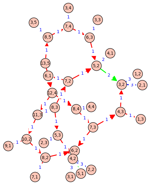
Call graph of a recursive function
def grafo_llamadas(f):
    class G(object):
        def __init__(self, f):
            self.f=f
            self.stack = []
            self.g   = DiGraph()
        def __call__(self, *args):
            if self.stack:
                sargs = ','.join(str(a) for a in args)
                last  = ','.join(str(a) for a in self.stack[-1])
                if self.g.has_edge(last, sargs):
                    l = self.g.edge_label(last, sargs)
                    self.g.set_edge_label(last, sargs, l + 1)
                else:
                    self.g.add_edge(last, sargs, 1)
            else:
                self.g   = DiGraph()
            self.stack.append(args)
            v = self.f(*args)
            self.stack.pop()
            return v
        def grafo(self):
            return self.g
    return G(f)

@grafo_llamadas
def particiones(n, k):
    if k == n:
        return [[1]*n]
    if k == 1:
        return [[n]]
    if not(0 < k < n):
        return []
    ls1 = [p+[1] for p in particiones(n-1, k-1)]
    ls2 = [[parte+1 for parte in p] for p in particiones(n-k, k)]
    return ls1 + ls2

particiones(13,5)
g = particiones.grafo()
g.show(edge_labels=True, figsize=(6,6), vertex_size=500, color_by_label=True)
# D3js interactive version
edge_partition = [
[edge for edge in g.edges() if edge[-1] == el]
for el in set(g.edge_labels())
]
g.show(method='js',
edge_labels=True,
vertex_labels=True,
link_distance=90,
charge=-400,
link_strength=2,
force_spring_layout=True,
edge_partition=edge_partition)
Sage plotting
Here are some python plotting engines/libraries:
- Older/not python dedicated:
Grace: grace, python interface
PLplot: http://www.plplot.org
opemath: Written by William Schelter and part of Maxima (thus also Sage) is a TCL/Tk plotting program which allows for interactive viewing. It has no separate download page. An example is this saddle: sage: maxima.eval("plot3d(2^(-u^2+v^2),[u,-1,1],[v,-1,1],[plot_format, openmath]);")
Dislin: dislin, disipyl (a python wrapper for dislin). It's license says dislin is "free for non-commercial use".
Pyqwt at http://pyqwt.sourceforge.net/ is a plotting package requiring QT. It seems to have some 3d capabilities http://pyqwt.sourceforge.net/pyqwt3d-examples.html.
matplotlib: http://matplotlib.sourceforge.net
Sage's plotting functionality is built on top of matplotlib, which is a very extensive plotting library with a user interface that is very similar to Matlab's plotting. The interface that Sage provides to matplotlib is very Mathematica like.
There are also several links to plotting/graphics/data visualization programs at the scipy wiki.

