|
Size: 8114
Comment: summarize #1321
|
Size: 15251
Comment: features in Sage 4.3.1.alpha2
|
| Deletions are marked like this. | Additions are marked like this. |
| Line 5: | Line 5: |
| * Substantial work towards a complete SPARC Solaris 10 port. This is due to the hard work of David Kirkby. The relevant tickets include [[http://trac.sagemath.org/sage_trac/ticket/6595 | #6595]], [[http://trac.sagemath.org/sage_trac/ticket/7138 | #7138]], [[http://trac.sagemath.org/sage_trac/ticket/7162 | #7162]], [[http://trac.sagemath.org/sage_trac/ticket/7505 | #7505]], [[http://trac.sagemath.org/sage_trac/ticket/7817 | #7817]]. | * Substantial work towards a complete SPARC Solaris 10 port. This is due to the hard work of David Kirkby. The relevant tickets include [[http://trac.sagemath.org/sage_trac/ticket/6595 | #6595]], [[http://trac.sagemath.org/sage_trac/ticket/7067 | #7067]], [[http://trac.sagemath.org/sage_trac/ticket/7138 | #7138]], [[http://trac.sagemath.org/sage_trac/ticket/7162 | #7162]], [[http://trac.sagemath.org/sage_trac/ticket/7387 | #7387]], [[http://trac.sagemath.org/sage_trac/ticket/7505 | #7505]], [[http://trac.sagemath.org/sage_trac/ticket/7817 | #7817]]. |
| Line 8: | Line 8: |
== Algebra == * [[http://trac.sagemath.org/sage_trac/ticket/7595 | #7595]] |
|
| Line 23: | Line 28: |
| * [[http://trac.sagemath.org/sage_trac/ticket/7739 | #7739]] |
|
| Line 25: | Line 33: |
| * [[http://trac.sagemath.org/sage_trac/ticket/7754 | #7754]] (Nicolas M. Thiéry) | * Weyl group optimizations [[http://trac.sagemath.org/sage_trac/ticket/7754 | #7754]] (Nicolas M. Thiéry) --- Three major improvements that indirectly also improve efficiency of most Weyl group routines: * Faster hash method calling the hash of the underlying matrix (which is set as immutable for that purpose). * New `__eq__()` method. * Action on the weight lattice realization: optimization of the matrix multiplication. Some operations are now up to 34% faster than previously: {{{ BEFORE sage: W = WeylGroup(["F", 4]) sage: W.cardinality() 1152 sage: %time list(W); CPU times: user 10.51 s, sys: 0.05 s, total: 10.56 s Wall time: 10.56 s sage: W = WeylGroup(["E", 8]) sage: %time W.long_element(); CPU times: user 1.47 s, sys: 0.00 s, total: 1.47 s Wall time: 1.47 s AFTER sage: W = WeylGroup(["F", 4]) sage: W.cardinality() 1152 sage: %time list(W); CPU times: user 6.89 s, sys: 0.04 s, total: 6.93 s Wall time: 6.93 s sage: W = WeylGroup(["E", 8]) sage: %time W.long_element(); CPU times: user 1.21 s, sys: 0.00 s, total: 1.21 s Wall time: 1.21 s }}} * [[http://trac.sagemath.org/sage_trac/ticket/7301 | #7301]] * [[http://trac.sagemath.org/sage_trac/ticket/7729 | #7729]] * [[http://trac.sagemath.org/sage_trac/ticket/7753 | #7753]] |
| Line 94: | Line 141: |
| * [[http://trac.sagemath.org/sage_trac/ticket/7724 | #7724]] (Nathann Cohen, Yann Laigle-Chapuy) * [[http://trac.sagemath.org/sage_trac/ticket/7770 | #7770]] (Rob Beezer) |
* Breadth/depth first searches and basic connectivity for c_graphs [[http://trac.sagemath.org/sage_trac/ticket/7724 | #7724]] (Nathann Cohen, Yann Laigle-Chapuy) --- Implementation of the following methods for the class `CGraphBackend` in the module `sage/graphs/base/c_graph.pyx`: * `depth_first_search()` * `breadth_first_search()` * `is_connected()` * `is_strongly_connected()` In some cases, the c_graphs implementation of these methods provides a 2x speed improvement: {{{ sage: g = graphs.RandomGNP(1000, 0.01) sage: h = g.copy(implementation="c_graph") sage: %timeit list(g.depth_first_search(0)); 100 loops, best of 3: 8.17 ms per loop sage: %timeit list(h.depth_first_search(0)); 100 loops, best of 3: 3.29 ms per loop sage: sage: %timeit list(g.breadth_first_search(0)); 100 loops, best of 3: 6.48 ms per loop sage: %timeit list(h.breadth_first_search(0)); 10 loops, best of 3: 34 ms per loop sage: sage: %timeit g.is_connected(); 100 loops, best of 3: 8.47 ms per loop sage: %timeit h.is_connected(); 100 loops, best of 3: 3.41 ms per loop sage: sage: g = g.to_directed() sage: h = g.copy(implementation="c_graph") sage: %timeit g.is_strongly_connected(); 10 loops, best of 3: 23.5 ms per loop sage: %timeit h.is_strongly_connected(); 10 loops, best of 3: 25 ms per loop }}} * Tower of Hanoi graph [[http://trac.sagemath.org/sage_trac/ticket/7770 | #7770]] (Rob Beezer) --- The Tower of Hanoi puzzle can be described by a graph whose vertices are possible states of the disks on the pegs, with edges representing legitimate moves of a single disk. The new method `HanoiTowerGraph()` of the class `GraphGenerators` in the module `sage/graphs/graph_generators.py` returns the graph whose vertices are the states of the Tower of Hanoi puzzle, with edges representing legal moves between states. See the documentation of this method for details on interpreting the the possible states of this puzzle. The following screenshot shows all the possible states of an instance of the puzzle with 3 pegs and 3 disks, produced using the following code: {{{ H = graphs.HanoiTowerGraph(3, 3, positions=False) show(H, figsize=[8,8]) }}} {{attachment:tower-hanoi-graph.png}} * [[http://trac.sagemath.org/sage_trac/ticket/7292 | #7292]] * [[http://trac.sagemath.org/sage_trac/ticket/7590 | #7590]] * [[http://trac.sagemath.org/sage_trac/ticket/7634 | #7634]] |
| Line 101: | Line 194: |
| * [[http://trac.sagemath.org/sage_trac/ticket/5174 | #5174]] (John Palmieri) | * Viewing entries of large matrices [[http://trac.sagemath.org/sage_trac/ticket/5174 | #5174]] (John Palmieri) --- For a small matrix such as `2 x 2`, the default is to print the entries of the matrix. This default behaviour is unsuitable for large matrices such as `100 x 100`. The string representation of such large matrices now indicate how to view all their entries. Here are some examples illustrating the new way to view the string representation of matrices. If the matrix is too big, all the elements are not displayed by default: {{{ sage: A = random_matrix(ZZ, 5) sage: A [ 1 -4 -4 1 -1] [-1 1 13 -1 -1] [-1 0 0 -1 -1] [-8 1 -1 1 -4] [ 1 -5 -1 1 2] sage: A = random_matrix(ZZ, 100) sage: A 100 x 100 dense matrix over Integer Ring (type 'print A.str()' to see all of the entries) }}} If a matrix has several names, refer to the matrix as "obj": {{{ sage: A = random_matrix(ZZ, 200) sage: B = A sage: B 200 x 200 dense matrix over Integer Ring (type 'print obj.str()' to see all of the entries) }}} If a matrix doesn't have a name, don't print any name referring to the matrix in its string representation: {{{ sage: A = random_matrix(ZZ, 150) sage: A.transpose() 150 x 150 dense matrix over Integer Ring sage: T = A.transpose(); T 150 x 150 dense matrix over Integer Ring (type 'print T.str()' to see all of the entries) }}} |
| Line 108: | Line 229: |
| * [[http://trac.sagemath.org/sage_trac/ticket/6820 | #6820]] (John Palmieri, Mitesh Patel) * [[http://trac.sagemath.org/sage_trac/ticket/7482 | #7482]] (William Stein) |
* Command line access to HTML documentation and docstrings [[http://trac.sagemath.org/sage_trac/ticket/6820 | #6820]] (John Palmieri, Mitesh Patel) --- Browse the Sage standard documentation from the command line or within the notebook interface. Use the following commands to browse documents in the standard documentation: * `browse_sage_doc.tutorial()` or its alias `tutorial()` * `browse_sage_doc.reference()`, or its aliases `reference()` and `manual()` * `browse_sage_doc.developer()` or its alias `developer()` * `browse_sage_doc.constructions()` or its alias `constructions()` The following screenshot illustrates viewing the Sage tutorial from the command line interface, activated using the command: {{{ sage: tutorial() }}} This command invoked a terminal-based web browser such as Links to view the tutorial. {{attachment:browse-doc-cmd.png}} * A mode for automatic names [[http://trac.sagemath.org/sage_trac/ticket/7482 | #7482]] (William Stein) --- Provide a mode so that undeclared variables magically spring into existence and object oriented notation is not necessary. The target audience is people wanting to simplify use of Sage for calculus for undergraduate students. This new mode currently only works within the notebook. The following screenshot illustates how to use the mode for automatic names. {{attachment:automatic-names.png}} |
| Line 114: | Line 248: |
| * [[http://trac.sagemath.org/sage_trac/ticket/7740 | #7740]] |
|
| Line 117: | Line 253: |
| * [[http://trac.sagemath.org/sage_trac/ticket/7271 | #7271]] (Martin Albrecht) * [[http://trac.sagemath.org/sage_trac/ticket/7388 | #7388]] (Robert Miller) * [[http://trac.sagemath.org/sage_trac/ticket/7483 | #7483]] (William Stein) |
* Upgrade [[http://polybori.sourceforge.net | PolyBoRi]] to latest upstream release version 0.6.3.r1647-20091028[[http://trac.sagemath.org/sage_trac/ticket/7271 | #7271]] (Martin Albrecht). * Upgrade [[http://www.mathe2.uni-bayreuth.de/stoll/programs |ratpoints]] to latest upstream release version 2.1.3 [[http://trac.sagemath.org/sage_trac/ticket/7388 | #7388]] (Robert Miller). |
| Line 125: | Line 259: |
| * [[http://trac.sagemath.org/sage_trac/ticket/7745 | #7745]] (Karl-Dieter Crisman) * [[http://trac.sagemath.org/sage_trac/ticket/7825 | #7825]] (Peter Jeremy) * [[http://trac.sagemath.org/sage_trac/ticket/7840 | #7840]] (William Stein) |
* Upgrade [[http://maxima.sourceforge.net | Maxima]] to latest upstream release version 5.20.1 [[http://trac.sagemath.org/sage_trac/ticket/7745 | #7745]] (Karl-Dieter Crisman). * Upgrade [[http://nb.sagemath.org | Sage Notebook]] to latest upstream release version 0.5 [[http://trac.sagemath.org/sage_trac/ticket/7785 | #7785]] (William Stein). * Update [[http://pari.math.u-bordeaux.fr | Pari/GP]] to version 2.3.3.p6 [[http://trac.sagemath.org/sage_trac/ticket/7825 | #7825]] (Peter Jeremy). * [[http://trac.sagemath.org/sage_trac/ticket/7856 | #7856]] * [[http://trac.sagemath.org/sage_trac/ticket/7067 | #7067]] * [[http://trac.sagemath.org/sage_trac/ticket/7239 | #7239]] * [[http://trac.sagemath.org/sage_trac/ticket/7387 | #7387]] * [[http://trac.sagemath.org/sage_trac/ticket/7761 | #7761]] * [[http://trac.sagemath.org/sage_trac/ticket/7814 | #7814]] |
Sage 4.3.1 Release Tour
Major features
Substantial work towards a complete SPARC Solaris 10 port. This is due to the hard work of David Kirkby. The relevant tickets include #6595, #7067, #7138, #7162, #7387, #7505, #7817.
We're moving closer towards a FreeBSD port, thanks to the work of Peter Jeremy at ticket #7825.
Algebra
Basic arithmetics
Implement conjugate() for RealDoubleElement #7834 (Dag Sverre Seljebotn) --- New method conjugate() in the class RealDoubleElement of the module sage/rings/real_double.pyx for returning the complex conjugate of a real number. This is consistent with conjugate() methods in ZZ and RR. For example,
sage: ZZ(5).conjugate()
5
sage: RR(5).conjugate()
5.00000000000000
sage: RDF(5).conjugate()
5.0
Combinatorics
Weyl group optimizations #7754 (Nicolas M. Thiéry) --- Three major improvements that indirectly also improve efficiency of most Weyl group routines:
- Faster hash method calling the hash of the underlying matrix (which is set as immutable for that purpose).
New __eq__() method.
- Action on the weight lattice realization: optimization of the matrix multiplication.
BEFORE

sage: W = WeylGroup(["F", 4])
sage: W.cardinality()
1152
sage: %time list(W);
CPU times: user 10.51 s, sys: 0.05 s, total: 10.56 s
Wall time: 10.56 s
sage: W = WeylGroup(["E", 8])
sage: %time W.long_element();
CPU times: user 1.47 s, sys: 0.00 s, total: 1.47 s
Wall time: 1.47 s


AFTER

sage: W = WeylGroup(["F", 4])
sage: W.cardinality()
1152
sage: %time list(W);
CPU times: user 6.89 s, sys: 0.04 s, total: 6.93 s
Wall time: 6.93 s
sage: W = WeylGroup(["E", 8])
sage: %time W.long_element();
CPU times: user 1.21 s, sys: 0.00 s, total: 1.21 s
Wall time: 1.21 s
Elliptic curves
Two-isogeny descent over QQ natively using ratpoints #6583 (Robert Miller) --- New module sage/schemes/elliptic_curves/descent_two_isogeny.pyx for descent on elliptic curves over QQ with a 2-isogeny. The relevant user interface function is two_descent_by_two_isogeny() that takes an elliptic curve E with a two-isogeny phi : E --> E' and dual isogeny phi', runs a two-isogeny descent on E, and returns n1, n2, n1' and n2'. Here, n1 is the number of quartic covers found with a rational point and n2 is the number which are ELS. Here are some examples illustrating the use of two_descent_by_two_isogeny():
sage: from sage.schemes.elliptic_curves.descent_two_isogeny import two_descent_by_two_isogeny
sage: E = EllipticCurve("14a")
sage: n1, n2, n1_prime, n2_prime = two_descent_by_two_isogeny(E)
sage: log(n1, 2) + log(n1_prime, 2) - 2  # the rank
0
sage: E = EllipticCurve("65a")
sage: n1, n2, n1_prime, n2_prime = two_descent_by_two_isogeny(E)
sage: log(n1, 2) + log(n1_prime, 2) - 2  # the rank
1
sage: E = EllipticCurve("1088j1")
sage: n1, n2, n1_prime, n2_prime = two_descent_by_two_isogeny(E)
sage: log(n1, 2) + log(n1_prime, 2) - 2  # the rank
2
You could also ask two_descent_by_two_isogeny() to be verbose in its computation:
sage: E = EllipticCurve("14a")
sage: two_descent_by_two_isogeny(E, verbosity=1)
2-isogeny
Results:
2 <= #E(Q)/phi'(E'(Q)) <= 2
2 <= #E'(Q)/phi(E(Q)) <= 2
#Sel^(phi')(E'/Q) = 2
#Sel^(phi)(E/Q) = 2
1 <= #Sha(E'/Q)[phi'] <= 1
1 <= #Sha(E/Q)[phi] <= 1
1 <= #Sha(E/Q)[2], #Sha(E'/Q)[2] <= 1
0 <= rank of E(Q) = rank of E'(Q) <= 0
(2, 2, 2, 2)
More functions for elliptic curve isogenies #6887 (John Cremona, Jenny Cooley) --- Code for constructing elliptic curve isogenies already existed in Sage 4.1.1. The enhancements here include:
For l=2,3,5,7,13 over any field, find all l-isogenies of a given elliptic curve. (These are the l for which X_0(l) has genus 0).
Similarly for the remaining l for which l-isogenies exist over QQ.
Given an elliptic curve over QQ, find the whole isogeny class in a robust manner.
Testing if two curves are isogenous at least over QQ.
The relevant use interface method is isogenies_prime_degree() in the class EllipticCurve_field of the module sage/schemes/elliptic_curves/ell_field.py. Here are some examples showing isogenies_prime_degree() in action. Examples over finite fields:
sage: E = EllipticCurve(GF(next_prime(1000000)), [7,8])
sage: E.isogenies_prime_degree()
[Isogeny of degree 2 from Elliptic Curve defined by y^2 = x^3 + 7*x + 8 over Finite Field of size 1000003 to Elliptic Curve defined by y^2 = x^3 + 970389*x + 794257 over Finite Field of size 1000003, Isogeny of degree 2 from Elliptic Curve defined by y^2 = x^3 + 7*x + 8 over Finite Field of size 1000003 to Elliptic Curve defined by y^2 = x^3 + 29783*x + 206196 over Finite Field of size 1000003, Isogeny of degree 2 from Elliptic Curve defined by y^2 = x^3 + 7*x + 8 over Finite Field of size 1000003 to Elliptic Curve defined by y^2 = x^3 + 999960*x + 78 over Finite Field of size 1000003, Isogeny of degree 13 from Elliptic Curve defined by y^2 = x^3 + 7*x + 8 over Finite Field of size 1000003 to Elliptic Curve defined by y^2 = x^3 + 878063*x + 845666 over Finite Field of size 1000003, Isogeny of degree 13 from Elliptic Curve defined by y^2 = x^3 + 7*x + 8 over Finite Field of size 1000003 to Elliptic Curve defined by y^2 = x^3 + 375648*x + 342776 over Finite Field of size 1000003]
sage: E.isogenies_prime_degree(13)
[Isogeny of degree 13 from Elliptic Curve defined by y^2 = x^3 + 7*x + 8 over Finite Field of size 1000003 to Elliptic Curve defined by y^2 = x^3 + 878063*x + 845666 over Finite Field of size 1000003, Isogeny of degree 13 from Elliptic Curve defined by y^2 = x^3 + 7*x + 8 over Finite Field of size 1000003 to Elliptic Curve defined by y^2 = x^3 + 375648*x + 342776 over Finite Field of size 1000003]
Examples over number fields (other than QQ):
sage: QQroot2.<e> = NumberField(x^2 - 2)
sage: E = EllipticCurve(QQroot2, [1,0,1,4,-6])
sage: E.isogenies_prime_degree(2)
[Isogeny of degree 2 from Elliptic Curve defined by y^2 + x*y + y = x^3 + 4*x + (-6) over Number Field in e with defining polynomial x^2 - 2 to Elliptic Curve defined by y^2 + x*y + y = x^3 + (-36)*x + (-70) over Number Field in e with defining polynomial x^2 - 2]
sage: E.isogenies_prime_degree(3)
[Isogeny of degree 3 from Elliptic Curve defined by y^2 + x*y + y = x^3 + 4*x + (-6) over Number Field in e with defining polynomial x^2 - 2 to Elliptic Curve defined by y^2 + x*y + y = x^3 + (-171)*x + (-874) over Number Field in e with defining polynomial x^2 - 2, Isogeny of degree 3 from Elliptic Curve defined by y^2 + x*y + y = x^3 + 4*x + (-6) over Number Field in e with defining polynomial x^2 - 2 to Elliptic Curve defined by y^2 + x*y + y = x^3 + (-128/3)*x + 5662/27 over Number Field in e with defining polynomial x^2 - 2]
Graph theory
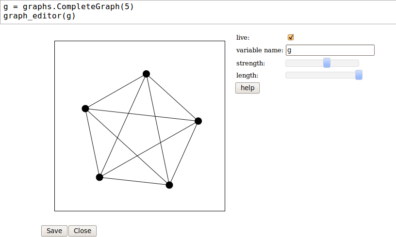
An interactive graph editor #1321 (Radoslav Kirov, Mitesh Patel) --- Embed an interactive graph editor into the notebook. The following screenshot shows a graph editor for playing around with the complete graph on 5 vertices:

Breadth/depth first searches and basic connectivity for c_graphs #7724 (Nathann Cohen, Yann Laigle-Chapuy) --- Implementation of the following methods for the class CGraphBackend in the module sage/graphs/base/c_graph.pyx:
depth_first_search()
breadth_first_search()
is_connected()
is_strongly_connected()
sage: g = graphs.RandomGNP(1000, 0.01)
sage: h = g.copy(implementation="c_graph")
sage: %timeit list(g.depth_first_search(0));
100 loops, best of 3: 8.17 ms per loop
sage: %timeit list(h.depth_first_search(0));
100 loops, best of 3: 3.29 ms per loop
sage:
sage: %timeit list(g.breadth_first_search(0));
100 loops, best of 3: 6.48 ms per loop
sage: %timeit list(h.breadth_first_search(0));
10 loops, best of 3: 34 ms per loop
sage:
sage: %timeit g.is_connected();
100 loops, best of 3: 8.47 ms per loop
sage: %timeit h.is_connected();
100 loops, best of 3: 3.41 ms per loop
sage:
sage: g = g.to_directed()
sage: h = g.copy(implementation="c_graph")
sage: %timeit g.is_strongly_connected();
10 loops, best of 3: 23.5 ms per loop
sage: %timeit h.is_strongly_connected();
10 loops, best of 3: 25 ms per loop
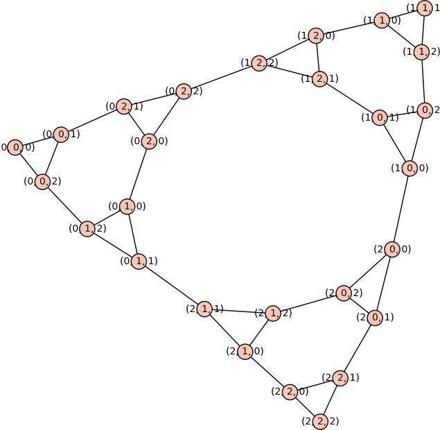
Tower of Hanoi graph #7770 (Rob Beezer) --- The Tower of Hanoi puzzle can be described by a graph whose vertices are possible states of the disks on the pegs, with edges representing legitimate moves of a single disk. The new method HanoiTowerGraph() of the class GraphGenerators in the module sage/graphs/graph_generators.py returns the graph whose vertices are the states of the Tower of Hanoi puzzle, with edges representing legal moves between states. See the documentation of this method for details on interpreting the the possible states of this puzzle. The following screenshot shows all the possible states of an instance of the puzzle with 3 pegs and 3 disks, produced using the following code:
H = graphs.HanoiTowerGraph(3, 3, positions=False)
show(H, figsize=[8,8])

Linear algebra
Viewing entries of large matrices #5174 (John Palmieri) --- For a small matrix such as 2 x 2, the default is to print the entries of the matrix. This default behaviour is unsuitable for large matrices such as 100 x 100. The string representation of such large matrices now indicate how to view all their entries. Here are some examples illustrating the new way to view the string representation of matrices. If the matrix is too big, all the elements are not displayed by default:
sage: A = random_matrix(ZZ, 5)
sage: A
[ 1 -4 -4  1 -1]
[-1  1 13 -1 -1]
[-1  0  0 -1 -1]
[-8  1 -1  1 -4]
[ 1 -5 -1  1  2]
sage: A = random_matrix(ZZ, 100)
sage: A
100 x 100 dense matrix over Integer Ring (type 'print A.str()' to see all of the entries)
If a matrix has several names, refer to the matrix as "obj":sage: A = random_matrix(ZZ, 200) sage: B = A sage: B 200 x 200 dense matrix over Integer Ring (type 'print obj.str()' to see all of the entries)
If a matrix doesn't have a name, don't print any name referring to the matrix in its string representation:sage: A = random_matrix(ZZ, 150) sage: A.transpose() 150 x 150 dense matrix over Integer Ring sage: T = A.transpose(); T 150 x 150 dense matrix over Integer Ring (type 'print T.str()' to see all of the entries)
#7728 (Dag Sverre Seljebotn)
Miscellaneous
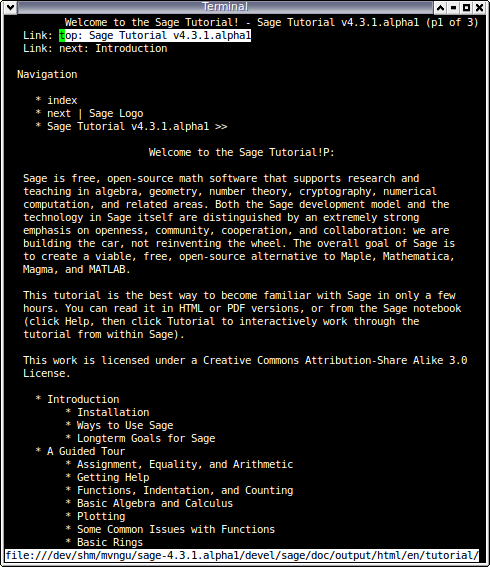
Command line access to HTML documentation and docstrings #6820 (John Palmieri, Mitesh Patel) --- Browse the Sage standard documentation from the command line or within the notebook interface. Use the following commands to browse documents in the standard documentation:
browse_sage_doc.tutorial() or its alias tutorial()
browse_sage_doc.reference(), or its aliases reference() and manual()
browse_sage_doc.developer() or its alias developer()
browse_sage_doc.constructions() or its alias constructions()
sage: tutorial()
This command invoked a terminal-based web browser such as Links to view the tutorial.
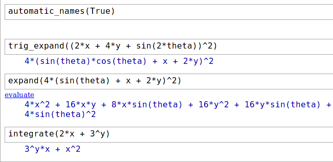
A mode for automatic names #7482 (William Stein) --- Provide a mode so that undeclared variables magically spring into existence and object oriented notation is not necessary. The target audience is people wanting to simplify use of Sage for calculus for undergraduate students. This new mode currently only works within the notebook. The following screenshot illustates how to use the mode for automatic names.

#7514 (William Stein)
Packages
Upgrade PolyBoRi to latest upstream release version 0.6.3.r1647-20091028#7271 (Martin Albrecht).
Upgrade ratpoints to latest upstream release version 2.1.3 #7388 (Robert Miller).
Upgrade Maxima to latest upstream release version 5.20.1 #7745 (Karl-Dieter Crisman).
Upgrade Sage Notebook to latest upstream release version 0.5 #7785 (William Stein).
