|
Size: 13918
Comment: Summarize #6000, #6167, #6093, #6050, #5931
|
Size: 19559
Comment: Summarize #5827
|
| Deletions are marked like this. | Additions are marked like this. |
| Line 271: | Line 271: |
| * Improve speed of combinatorial algebra multiplication (Dan Christensen) -- The speed-up concerns the method {{{multiply()}}} of the class {{{CombinatorialAlgebra}}} in {{{sage/combinat/combinatorial_algebra.py}}}. == Commutative Algebra == * FIXME: summarize #6120 |
* Improve speed of combinatorial algebra multiplication (Dan Christensen) -- The speed-up concerns the method {{{multiply()}}} of the class {{{CombinatorialAlgebra}}} in {{{sage/combinat/combinatorial_algebra.py}}}. The speed-up can be up to ... |
| Line 291: | Line 285: |
| * FIXME: summarize #5599 |
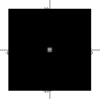
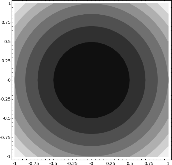
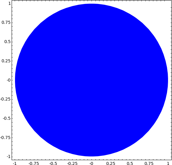
* Centering of contour and density plots (Jason Grout) -- The following example shows a "spotlight" on the origin: {{{ sage: x, y = var('x,y') sage: density_plot(1/(x^10+y^10), (x, -10, 10), (y, -10, 10)) }}} {{attachment:spotlight.png}} This plots concentric circles centered at the origin: {{{ sage: x, y = var('x,y') sage: contour_plot(x^2 + y^2 - 2, (x,-1,1), (y,-1,1)).show(aspect_ratio=1) }}} {{attachment:concentric-circles.png}} The following example plots a disk centered at the origin: {{{ sage: x, y = var('x,y') sage: region_plot(x^2 + y^2 < 1, (x,-1,1), (y,-1,1)).show(aspect_ratio=1) }}} {{attachment:disk.png}} |
| Line 329: | Line 342: |
| * FIXME: summarize #5967 * FIXME: summarize #5483 * FIXME: summarize #6139 |
* Wrapping Sage or Python objects as Sage elements (Nicolas Thiery) -- New class {{{ElementWrapper}}} in {{{sage/structure/element_wrapper.py}}} for wrapping Sage or Python objects as Sage elements, with reasonable default implementations of {{{repr}}}, {{{cmp}}}, {{{hash}}}, etc. The typical use case is for trivially constructing new element classes from pre-existing Sage or Python classes, with a containment relation. Here's an example on using {{{ElementWrapper}}}: {{{ sage: o = ElementWrapper("bla", parent=ZZ); o 'bla' sage: isinstance(o, sage.structure.element.Element) True sage: o.parent() Integer Ring sage: o.value 'bla' }}} * A tool for understanding Python pickles (Carl Witty) -- The new module {{{sage/misc/explain_pickle.py}}} has a function called {{{explain_pickle}}} that takes a pickle and produces Sage code that will evaluate to the contents of the pickle. The combination of {{{explain_sage}}} to produce Sage code and {{{sage_eval}}} to evaluate the code should be a 100% compatible implementation of cPickle's unpickler. That is, {{{explain_sage}}} explains a pickle by producing source code such that evaluating the code is equivalent to loading the pickle. Feeding the result of {{{explain_pickle}}} to {{{sage_eval}}} should be totally equivalent to loading the pickle with cPickle. Here are some examples on using {{{explain_pickle}}}: {{{ sage: explain_pickle(dumps({('a', 'b'): [1r, 2r]})) {('a', 'b'):[1r, 2r]} sage: explain_pickle(dumps(RR(pi)), in_current_sage=True) from sage.rings.real_mpfr import __create__RealNumber_version0 from sage.rings.real_mpfr import __create__RealField_version0 __create__RealNumber_version0(__create__RealField_version0(53r, False, 'RNDN'), '3.4gvml245kc0@0', 32r) sage: s = 'hi' sage: explain_pickle(dumps((s, s))) ('hi', 'hi') sage: explain_pickle(dumps((s, s)), pedantic=True) si = 'hi' (si, si) sage: explain_pickle(dumps(5r) ....: ) 5r sage: explain_pickle(dumps(22/7)) pg_make_rational = unpickle_global('sage.rings.rational', 'make_rational') pg_make_rational('m/7') sage: explain_pickle(dumps(22/7), in_current_sage=True) from sage.rings.rational import make_rational make_rational('m/7') sage: explain_pickle(dumps(22/7), default_assumptions=True) from sage.rings.rational import make_rational make_rational('m/7') }}} * S-box calling when {{{m != n}}} (Martin Albrecht) -- An S-box takes {{{m}}} input bits and transforms them into {{{n}}} output bits. This is called an {{{m x n}}} S-box. The case of invoking an S-box with {{{m != n}}} is now supported: {{{ sage: S = mq.SBox(3, 0, 1, 3, 1, 0, 2, 2) sage: S(0) 3 sage: S([0,0,0]) [1, 1] }}} |
| Line 339: | Line 402: |
| * FIXME: summarize #5995 | * Membership testing for modular forms subspaces (David Loeffler) -- One can test such membership as follows: {{{ sage: M = ModularForms(17, 4) sage: S = M.cuspidal_submodule() sage: M.0 == S.0 True sage: M.0 in S True }}} |
| Line 345: | Line 416: |
| * FIXME: summarize #4575 * FIXME: summarize #5895 |
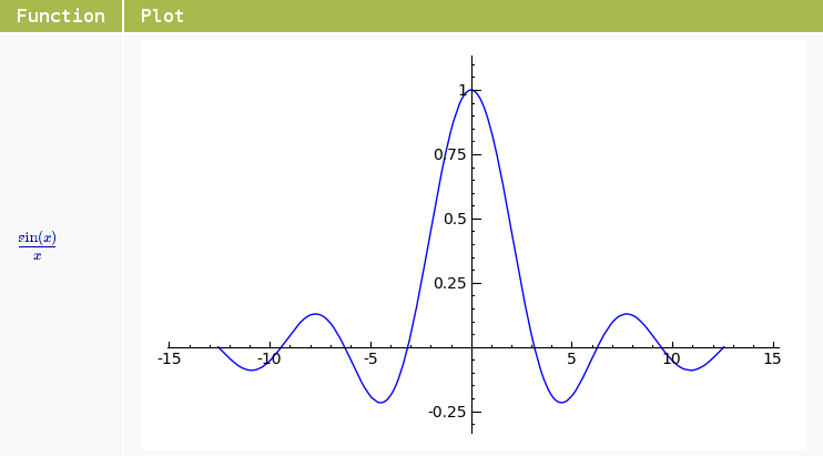
* Show nested lists as HTML tables (Wilfried Huss) -- One can produce such HTML tables as follows: {{{ sage: functions = [sin(x), cos(x), tan(x), acos(x)] sage: t = [[f, taylor(f, x, 0, 10)] for f in functions] sage: html.table([["Function", "Series"]] + t, header = True) }}} {{attachment:html-table-1.png}} One can also place graphic objects into the table: {{{ sage: f = 1/x*sin(x) sage: t = [["Function", "Plot"],[f, plot(f, x, -4*pi, 4*pi)]] sage: html.table(t, header = True) }}} {{attachment:html-table-2.png}} * Limit the number of worksheet snapshots (Rob Beezer) -- Reduce the unlimited growth of snapshots of worksheets when using the notebook. |
| Line 353: | Line 438: |
| * FIXME: summarize #133 * FIXME: summarize #6021 * FIXME: summarize #6206 |
* Galois action (David Loeffler) -- For example, one can now perform computations similar to the following: {{{ sage: F.<z> = CyclotomicField(7) sage: G = F.galois_group() sage: phi = G.random_element() sage: phi(z) z^4 }}} * Period lattices for elliptic curves over {{{CC}}} (John Cremona) -- For elliptic curves over number fields, period lattice for complex embeddings is supported, using the complex AGM (Gauss' Arithmetic-Geometric Mean) method to compute the basis. Here's an example: {{{ sage: K.<a> = NumberField(x^3 - 2) sage: E = EllipticCurve([0, 1, 0, a, a]) sage: emb = K.embeddings(ComplexField())[0] sage: E.period_lattice(emb) Period lattice associated to Elliptic Curve defined by y^2 = x^3 + x^2 + a*x + a over Number Field in a with defining polynomial x^3 - 2 with respect to the embedding Ring morphism: From: Number Field in a with defining polynomial x^3 - 2 To: Algebraic Field Defn: a |--> -0.6299605249474365? - 1.091123635971722?*I }}} * Move the {{{algebraic_closure}}} method from {{{RLF}}} to {{{LazyField}}} (Nick Alexander). |
| Line 363: | Line 468: |
| * FIXME: summarize #5827 | * Solving the subset sum problem for super-increasing sequences (Minh Van Nguyen) -- New module {{{sage/numerical/knapsack.py}}} for solving knapsack problems. The class {{{Superincreasing}}} in that module can be used to solve the subset sum problem for super-increasing sequences. Here are some examples: {{{ sage: from sage.numerical.knapsack import Superincreasing sage: L = [1, 2, 5, 21, 69, 189, 376, 919] sage: seq = Superincreasing(L) sage: seq Super-increasing sequence of length 8 sage: seq.is_superincreasing() True sage: Superincreasing().is_superincreasing([1,3,5,7]) False }}} |
Sage 4.0.1 Release Tour
Sage 4.0.1 was released on FIXME. For the official, comprehensive release note, please refer to FIXME. A nicely formatted version of this release tour can be found at FIXME. The following points are some of the foci of this release:
Algebra
Factoring rational functions (Soroosh Yazdani) -- New method factor() in the class FractionFieldElement of sage/rings/fraction_field_element.pyx to return the factorization of self over the base ring. Here's an example for working with this new method:
sage: K.<x> = QQ["x"]
sage: f = (x^3 + x) / (x-3)
sage: f.factor()
(x - 3)^-1 * x * (x^2 + 1)
Faster basis_matrix() for ambient modules (John Cremona) -- The speed-up can be up to 376x faster than previously. The following timing statistics were obtained using the machine sage.math:
# BEFORE

sage: K = FreeModule(ZZ, 2000)
sage: %time I = K.basis_matrix()
CPU times: user 292.74 s, sys: 20.11 s, total: 312.85 s
Wall time: 312.90 s


# AFTER

sage: K = FreeModule(ZZ, 2000)
sage: %time I = K.basis_matrix()
CPU times: user 0.41 s, sys: 0.43 s, total: 0.84 s
Wall time: 0.83 s
Optimize the construction of Lagrange interpolation polynomials (Minh Van Nguyen) -- Rewrite the method lagrange_polynomial() in the class PolynomialRing_field of sage/rings/polynomial/polynomial_ring.py for generating the n-th Lagrange interpolation polynomial. The method now provides two new options:
algorithm --- (default: divided_difference) If algorithm="divided_difference", then use the method of divided difference. If algorithm="neville", then use a variant of Neville's method to recursively generate the n-th Lagrange interpolation polynomial. This adaptation of Neville's method is more memory efficient than the original Neville's method, since the former doesn't generate the full Neville table resulting from Neville's recursive procedure. Instead the adaptation only keeps track of the current and previous rows of the said table.
previous_row --- (default: None) This is only relevant if used together with algorithm="neville". Here "previous row" refers to the last row in the Neville table that was obtained from a previous computation of an n-th Lagrange interpolation polynomial using Neville's method. If the last row is provided, then use a memory efficient variant of Neville's method to recursively generate a better interpolation polynomial from the results of previous computation.
There's also the new method divided_difference() to compute the Newton divided-difference coefficients of the n-th Lagrange interpolation polynomial. The following are some timing statistics obtained using sage.math. When the results of previous computations are fed to lagrange_polynomial in order to produce better interpolation polynomials, we can gain an efficiency of up to 42%.
# BEFORE

# using the definition of Lagrange interpolation polynomial
sage: R = PolynomialRing(QQ, 'x')
sage: %timeit R.lagrange_polynomial([(0,1),(2,2),(3,-2),(-4,9)])
1000 loops, best of 3: 1.71 ms per loop
sage: R = PolynomialRing(GF(2**3,'a'), 'x')
sage: a = R.base_ring().gen()
sage: timeit("R.lagrange_polynomial([(a^2+a,a),(a,1),(a^2,a^2+a+1)])")
625 loops, best of 3: 233 µs per loop

# without using precomputed values to generate successively better interpolation polynomials

sage: R = PolynomialRing(QQ, 'x')
sage: timeit("R.lagrange_polynomial([(0,1),(2,2)])");
625 loops, best of 3: 571 µs per loop
sage: # add two more points
sage: timeit("R.lagrange_polynomial([(0,1),(2,2),(3,-2),(-4,9)])");
125 loops, best of 3: 2.29 ms per loop
sage:
sage: R = PolynomialRing(GF(2**3,'a'), 'x')
sage: a = R.base_ring().gen()
sage: timeit("R.lagrange_polynomial([(a^2+a,a),(a,1)])")
625 loops, best of 3: 76.1 µs per loop
sage: # add another point
sage: timeit("R.lagrange_polynomial([(a^2+a,a),(a,1),(a^2,a^2+a+1)])")
625 loops, best of 3: 229 µs per loop
sage:
sage: R = PolynomialRing(QQ, 'x')
sage: points = [(random(), random()) for i in xrange(100)]
sage: time R.lagrange_polynomial(points);
CPU times: user 1.21 s, sys: 0.00 s, total: 1.21 s
Wall time: 1.21 s
sage: # add three more points
sage: for i in xrange(3): points.append((random(), random()))
....:
sage: time R.lagrange_polynomial(points);
CPU times: user 1.28 s, sys: 0.01 s, total: 1.29 s
Wall time: 1.29 s
sage: # add another 100 points
sage: for i in xrange(100): points.append((random(), random()))
....:
sage: time R.lagrange_polynomial(points);
CPU times: user 5.87 s, sys: 0.02 s, total: 5.89 s
Wall time: 5.89 s


# AFTER

# using the method of divided-difference
sage: R = PolynomialRing(QQ, 'x')
sage: %timeit R.lagrange_polynomial([(0,1),(2,2),(3,-2),(-4,9)])
1000 loops, best of 3: 827 µs per loop
sage: R = PolynomialRing(GF(2**3,'a'), 'x')
sage: a = R.base_ring().gen()
sage: timeit("R.lagrange_polynomial([(a^2+a,a),(a,1),(a^2,a^2+a+1)])")
625 loops, best of 3: 111 µs per loop

# using precomputed values to generate successively better interpolation polynomials

sage: R = PolynomialRing(QQ, 'x')
sage: timeit("R.lagrange_polynomial([(0,1),(2,2)], neville=True)");
625 loops, best of 3: 332 µs per loop
sage: p = R.lagrange_polynomial([(0,1),(2,2)], neville=True);
sage: # add two more points
sage: timeit("R.lagrange_polynomial([(0,1),(2,2),(3,-2),(-4,9)], neville=True, previous_row=p)");
625 loops, best of 3: 1.41 ms per loop
sage:
sage: R = PolynomialRing(GF(2**3,'a'), 'x')
sage: a = R.base_ring().gen()
sage: timeit("R.lagrange_polynomial([(a^2+a,a),(a,1)], neville=True)");
625 loops, best of 3: 36.4 µs per loop
sage: p = R.lagrange_polynomial([(a^2+a,a),(a,1)], neville=True);
sage: # add another point
sage: timeit("R.lagrange_polynomial([(a^2+a,a),(a,1),(a^2,a^2+a+1)], neville=True, previous_row=p)");
625 loops, best of 3: 131 µs per loop
sage:
sage: R = PolynomialRing(QQ, 'x')
sage: points = [(random(), random()) for i in xrange(100)]
sage: time R.lagrange_polynomial(points, neville=True);
CPU times: user 1.26 s, sys: 0.00 s, total: 1.26 s
Wall time: 1.26 s
sage: p = R.lagrange_polynomial(points, neville=True);
sage: # add three more points
sage: for i in xrange(3): points.append((random(), random()))
....:
sage: time R.lagrange_polynomial(points, neville=True, previous_row=p);
CPU times: user 0.09 s, sys: 0.00 s, total: 0.09 s
Wall time: 0.08 s
sage: p = R.lagrange_polynomial(points, neville=True, previous_row=p)
sage: # add another 100 points
sage: for i in xrange(100): points.append((random(), random()))
....:
sage: time R.lagrange_polynomial(points, neville=True, previous_row=p);
CPU times: user 4.62 s, sys: 0.00 s, total: 4.62 s
Wall time: 4.62 s
Algebraic Geometry
- FIXME: summarize #5948
Basic Arithmetic
Speed overhaul for digits, exact_log and ndigits (Joel B. Mohler) -- Speed-up for the cases where the method exact_log can conveniently be computed by log 2 estimation. In some cases, time efficiency can be up to 927x faster than previously. The following timing statistics were obtained using the machine sage.math:
# BEFORE

sage: n = 5^1000
sage: m = 2975982357823879528793587928793592
sage: %timeit n.exact_log(m)
1000 loops, best of 3: 205 µs per loop
sage: n = 5^50
sage: m = 33
sage: %timeit n.exact_log(m)
10000 loops, best of 3: 29.6 µs per loop
sage: def zlog(m, n, k):
....:     for i in xrange(0, m/1000):
....:         a = ZZ.random_element(n) + 2
....:         b = ZZ.random_element(k)
....:         c = a^b
....:         for i in xrange (0, 1000):
....:             c.exact_log(a)
....:
sage: time zlog(100000, 2^100, 100)
CPU times: user 22.59 s, sys: 0.12 s, total: 22.71 s
Wall time: 22.70 s
sage: time zlog(100000, 100, 100)
CPU times: user 3.45 s, sys: 0.02 s, total: 3.47 s
Wall time: 3.47 s


# AFTER

sage: n = 5^1000
sage: m = 2975982357823879528793587928793592
sage: %timeit n.exact_log(m)
1000000 loops, best of 3: 221 ns per loop
sage: n = 5^50
sage: m = 33
sage: %timeit n.exact_log(m)
1000000 loops, best of 3: 526 ns per loop
sage: def zlog(m, n, k):
....:     for i in xrange(0, m/1000):
....:         a = ZZ.random_element(n) + 2
....:         b = ZZ.random_element(k)
....:         c = a^b
....:         for i in xrange (0, 1000):
....:             c.exact_log(a)
....:
sage: time zlog(100000, 2^100, 100)
CPU times: user 1.96 s, sys: 0.02 s, total: 1.98 s
Wall time: 1.99 s
sage: time zlog(100000, 100, 100)
CPU times: user 0.05 s, sys: 0.01 s, total: 0.06 s
Wall time: 0.05 s
Calculus
Deprecate the function numerical_sqrt() (Robert Bradshaw, John H. Palmieri) -- The function numerical_sqrt() in sage/misc/functional.py is now deprecated. Users are advised to instead use sqrt().
Combinatorics
Sets enumerated by exploring a search space with a (lazy) tree or graph structure (Nicolas Thiery) -- Extend the sage.combinat.backtrack library with other generic tools for constructing large sets whose elements can be enumerated by exploring a search space with a (lazy) tree or graph structure. The following generic utilities have been added:
SearchForest: Depth first search through a tree descrived by a "child" function.
GenericBacktracker: Depth first search through a tree descrived by a "child" function, with branch pruning, etc.
TransitiveIdeal: Depth first search through a graph described by a "neighbours" relation.
TransitiveIdealGraded: Breath first search through a graph described by a "neighbours" relation.
The Sloane sequence A000008 (Joanna Gaski) -- The Sloane sequence A000008 is concerned with the number of ways of making change for n cents where one is restricted to using only coins of denominations 1, 2, 5, and 10 cents. This is contained in the new class A000008 in sage/combinat/sloane_functions.py. Here are some examples on using this class:
sage: a = sloane.A000008; a
Number of ways of making change for n cents using coins of 1, 2, 5, 10 cents.
sage: a(0)
1
sage: a(1)
1
sage: a(13)
16
sage: a.list(14)
[1, 1, 2, 2, 3, 4, 5, 6, 7, 8, 11, 12, 15, 16]
Read ext_rep format of combinatorial designs (Carlo Hamalainen) -- The new module sage/combinat/designs/ext_rep.py is an API to the abstract tree represented by an XML document containing the External Representation of a list of block designs. The relevant combinatorial designs are read from the online database at http://designtheory.org/database. This module also provides the related I/O operations for reading and writing ext-rep files or data. The parsing is based on expat.
- Dynkin diagram ASCII art for reducible Cartan types (Dan Bump) -- Here are some examples on such ASCII art:
sage: CartanType("F4xA2").dynkin_diagram() O---O=>=O---O 1 2 3 4 O---O 5 6 F4xA2 sage: t = CartanType("A2xB2xF4") sage: dd = DynkinDiagram(t); dd O---O 1 2 O=>=O 3 4 O---O=>=O---O 5 6 7 8 A2xB2xF4 - Speed-up computation in symmetric algebra group (Dan Christensen) -- The previous code essentially reimplemented the multiplication in the group algebra. Now it accumulates the symmetrizers and antisymmetrizers separately, and then does one multiplication at the end. This probably results in the same number of operations, but it avoids creating many intermediate objects. The speed-up can be up to ...
Improve speed of combinatorial algebra multiplication (Dan Christensen) -- The speed-up concerns the method multiply() of the class CombinatorialAlgebra in sage/combinat/combinatorial_algebra.py. The speed-up can be up to ...
Geometry
Graph Theory
Graphics
- FIXME: summarize #6184
- Centering of contour and density plots (Jason Grout) -- The following example shows a "spotlight" on the origin:
sage: x, y = var('x,y')
sage: density_plot(1/(x^10+y^10), (x, -10, 10), (y, -10, 10))

- This plots concentric circles centered at the origin:
sage: x, y = var('x,y')
sage: contour_plot(x^2 + y^2 - 2, (x,-1,1), (y,-1,1)).show(aspect_ratio=1)

- The following example plots a disk centered at the origin:
sage: x, y = var('x,y')
sage: region_plot(x^2 + y^2 < 1, (x,-1,1), (y,-1,1)).show(aspect_ratio=1)

Group Theory
Interfaces
- Improving the GAP interface by pre-compiling certain regular expressions (Simon King) -- The speed-up in the GAP interface is now up to 37% faster than previously. The following timing statistics were obtained using the machine sage.math:
# BEFORE

sage: G = SymmetricGroup(7)
sage: g = G._gap_()
sage: l = g.Elements()
sage: time L = [gap.eval(l.name() + '[%d]^2' % (i)) for i in xrange(1, 7.factorial() + 1)]
CPU times: user 1.90 s, sys: 0.16 s, total: 2.06 s
Wall time: 2.08 s


# AFTER

sage: G = SymmetricGroup(7)
sage: g = G._gap_()
sage: l = g.Elements()
sage: time L = [gap.eval(l.name() + '[%d]^2' % (i)) for i in xrange(1, 7.factorial() + 1)]
CPU times: user 1.07 s, sys: 0.22 s, total: 1.29 s
Wall time: 1.31 s
Linear Algebra
Miscellaneous
Wrapping Sage or Python objects as Sage elements (Nicolas Thiery) -- New class ElementWrapper in sage/structure/element_wrapper.py for wrapping Sage or Python objects as Sage elements, with reasonable default implementations of repr, cmp, hash, etc. The typical use case is for trivially constructing new element classes from pre-existing Sage or Python classes, with a containment relation. Here's an example on using ElementWrapper:
sage: o = ElementWrapper("bla", parent=ZZ); o
'bla'
sage: isinstance(o, sage.structure.element.Element)
True
sage: o.parent()
Integer Ring
sage: o.value
'bla'
A tool for understanding Python pickles (Carl Witty) -- The new module sage/misc/explain_pickle.py has a function called explain_pickle that takes a pickle and produces Sage code that will evaluate to the contents of the pickle. The combination of explain_sage to produce Sage code and sage_eval to evaluate the code should be a 100% compatible implementation of cPickle's unpickler. That is, explain_sage explains a pickle by producing source code such that evaluating the code is equivalent to loading the pickle. Feeding the result of explain_pickle to sage_eval should be totally equivalent to loading the pickle with cPickle. Here are some examples on using explain_pickle:
sage: explain_pickle(dumps({('a', 'b'): [1r, 2r]}))
{('a', 'b'):[1r, 2r]}
sage: explain_pickle(dumps(RR(pi)), in_current_sage=True)

from sage.rings.real_mpfr import __create__RealNumber_version0
from sage.rings.real_mpfr import __create__RealField_version0
__create__RealNumber_version0(__create__RealField_version0(53r, False, 'RNDN'), '3.4gvml245kc0@0', 32r)
sage: s = 'hi'
sage: explain_pickle(dumps((s, s)))
('hi', 'hi')
sage: explain_pickle(dumps((s, s)), pedantic=True)

si = 'hi'
(si, si)
sage: explain_pickle(dumps(5r)
....: )
5r
sage: explain_pickle(dumps(22/7))

pg_make_rational = unpickle_global('sage.rings.rational', 'make_rational')
pg_make_rational('m/7')
sage: explain_pickle(dumps(22/7), in_current_sage=True)

from sage.rings.rational import make_rational
make_rational('m/7')
sage: explain_pickle(dumps(22/7), default_assumptions=True)

from sage.rings.rational import make_rational
make_rational('m/7')
S-box calling when m != n (Martin Albrecht) -- An S-box takes m input bits and transforms them into n output bits. This is called an m x n S-box. The case of invoking an S-box with m != n is now supported:
sage: S = mq.SBox(3, 0, 1, 3, 1, 0, 2, 2)
sage: S(0)
3
sage: S([0,0,0])
[1, 1]
Modular Forms
- Membership testing for modular forms subspaces (David Loeffler) -- One can test such membership as follows:
sage: M = ModularForms(17, 4)
sage: S = M.cuspidal_submodule()
sage: M.0 == S.0
True
sage: M.0 in S
True
Notebook
- Show nested lists as HTML tables (Wilfried Huss) -- One can produce such HTML tables as follows:
sage: functions = [sin(x), cos(x), tan(x), acos(x)]
sage: t = [[f, taylor(f, x, 0, 10)] for f in functions]
sage: html.table([["Function", "Series"]] + t, header = True)

- One can also place graphic objects into the table:
sage: f = 1/x*sin(x)
sage: t = [["Function", "Plot"],[f, plot(f, x, -4*pi, 4*pi)]]
sage: html.table(t, header = True)

- Limit the number of worksheet snapshots (Rob Beezer) -- Reduce the unlimited growth of snapshots of worksheets when using the notebook.
Number Theory
- Galois action (David Loeffler) -- For example, one can now perform computations similar to the following:
sage: F.<z> = CyclotomicField(7)
sage: G = F.galois_group()
sage: phi = G.random_element()
sage: phi(z)
z^4
Period lattices for elliptic curves over CC (John Cremona) -- For elliptic curves over number fields, period lattice for complex embeddings is supported, using the complex AGM (Gauss' Arithmetic-Geometric Mean) method to compute the basis. Here's an example:
sage: K.<a> = NumberField(x^3 - 2)
sage: E = EllipticCurve([0, 1, 0, a, a])
sage: emb = K.embeddings(ComplexField())[0]
sage: E.period_lattice(emb)

Period lattice associated to Elliptic Curve defined by y^2 = x^3 + x^2 + a*x + a over Number Field in a with defining polynomial x^3 - 2 with respect to the embedding Ring morphism:
  From: Number Field in a with defining polynomial x^3 - 2
  To:   Algebraic Field
  Defn: a |--> -0.6299605249474365? - 1.091123635971722?*I
Move the algebraic_closure method from RLF to LazyField (Nick Alexander).
Numerical
Solving the subset sum problem for super-increasing sequences (Minh Van Nguyen) -- New module sage/numerical/knapsack.py for solving knapsack problems. The class Superincreasing in that module can be used to solve the subset sum problem for super-increasing sequences. Here are some examples:
sage: from sage.numerical.knapsack import Superincreasing
sage: L = [1, 2, 5, 21, 69, 189, 376, 919]
sage: seq = Superincreasing(L)
sage: seq
Super-increasing sequence of length 8
sage: seq.is_superincreasing()
True
sage: Superincreasing().is_superincreasing([1,3,5,7])
False
Packages
- FIXME: summarize #5840
- FIXME: summarize #6173
- FIXME: summarize #5817
- FIXME: summarize #6156
- FIXME: summarize #6169
- FIXME: summarize #6209
- FIXME: summarize #6219
P-adics
Quadratic Forms
Symbolics
- FIXME: summarize #6144
- FIXME: summarize #6194
Topology
- FIXME: summarize #6141
