|
Size: 48544
Comment:
|
Size: 48544
Comment: Fix typo
|
| Deletions are marked like this. | Additions are marked like this. |
| Line 368: | Line 368: |
| The functions {{{iterator()}}} and {{{count()}}} are deprecated (with a warning), but will be removed in a later release. On the other hand, there was no way to keep backward compatibility for {{{len}}}. Indeed, many of function such as {{{list / filter / map}}} try silently to call {{{len}}}, which would have caused miriads of warnings to be issued in seemingly unrelated places. So it was decided to simply remove it and issue an error, suggesting to call {{{cardinality}}} instead. | The functions {{{iterator()}}} and {{{count()}}} are deprecated (with a warning), but will be removed in a later release. On the other hand, there was no way to keep backward compatibility for {{{len}}}. Indeed, many of function such as {{{list / filter / map}}} try silently to call {{{len}}}, which would have caused myriads of warnings to be issued in seemingly unrelated places. So it was decided to simply remove it and issue an error, suggesting to call {{{cardinality}}} instead. |
Sage 3.4.1 Release Tour
Sage 3.4.1 was released on April 22nd, 2009. For the official, comprehensive release note, please refer to sage-3.4.1.txt. A nicely formatted version of this release tour can be found at FIXME. The following points are some of the foci of this release:
- Upgrade to Cython 0.11.
Rewrite fast_float to support more data types.
- Improved UTF8/Unicode support in the Notebook.
- Latest upstream versions of MPIR and FLINT.
- Pizer's algorithm for computing Brandt Modules and Brandt Matrices.
- Quadratic twists for p-adic L-functions.
- Overconvergent modular forms for genus 0 primes.
- Many improvements for computing with number field.
Algebra
Optimized is_primitive() method (Ryan Hinton) -- The method is_primitive() in sage/rings/polynomial/polynomial_element.pyx is used for determining whether or not a polynomial is primitive over a finite field. Prime divisors are calculated during the test for polynomial primitivity. Where n is large, calculating those prime divisors can dominate the running time of the test. The is_primitive() method now has the optional argument n_prime_divs for providing precomputed prime divisors. This optional argument can result in a performance improvement of up to 4x. On the machine sage.math, one has the following timing statistics:
sage: R.<x> = PolynomialRing(GF(2), 'x')
sage: nn = 128
sage: max_order = 2^nn - 1
sage: pdivs = max_order.prime_divisors()
sage: poly = R.random_element(nn)
sage: while not (poly.degree()==nn and poly.is_primitive(max_order, pdivs)):
....:     poly = R.random_element(nn)
....:
sage: %timeit poly.is_primitive()  # without n_prime_divs optional argument
10 loops, best of 3: 285 ms per loop
sage: %timeit poly.is_primitive(max_order, pdivs)  # with n_prime_divs optional argument
10 loops, best of 3: 279 ms per loop
sage:
sage: nn = 256
sage: max_order = 2^nn - 1
sage: pdivs = max_order.prime_divisors()
sage: poly = R.random_element(nn)
sage: while not (poly.degree()==nn and poly.is_primitive(max_order, pdivs)):
....:     poly = R.random_element(nn)
....:
sage: %timeit poly.is_primitive()  # without n_prime_divs optional argument
10 loops, best of 3: 3.22 s per loop
sage: %timeit poly.is_primitive(max_order, pdivs)  # with n_prime_divs optional argument
10 loops, best of 3: 700 ms per loop
Speed-up the method order_from_multiple() (John Cremona) -- For groups of prime order n, every non-identity element has order n. The previous implementation of the method order_from_multiple() computes g^n twice when g is not the identity and n is prime. Such double computation is now avoided. Now for each prime p dividing the given multiple of the order, we avoid the last multiplication/powering by p, hence saving some computation time whenever the p-exponent of the order is maximal. The new implementation of order_from_multiple() results in a performance improvement of up to 25%. Here are some timing statistics obtained using the machine sage.math:
# BEFORE

sage: F = GF(2^1279, 'a')
sage: n = F.cardinality() - 1 # Mersenne prime
sage: order_from_multiple(F.random_element(), n, [n], operation='*') == n
True
sage: %timeit order_from_multiple(F.random_element(), n, [n], operation='*') == n
10 loops, best of 3: 63.7 ms per loop


# AFTER

sage: F = GF(2^1279, 'a')
sage: n = F.cardinality() - 1 # Mersenne prime
sage: %timeit order_from_multiple(F.random_element(), n, [n], operation='*') == n
10 loops, best of 3: 47.2 ms per loop
Speed-up in irreducibility test (Ryan Hinton) -- For polynomials over the finite field GF(2), the test for irreducibility is now up to 40,000 times faster than previously. On a 64-bit Debian/squeeze machine with Core 2 Duo running at 2.33 GHz, one has the following timing improvements:
# BEFORE

sage: P.<x> = GF(2)[]
sage: f = P.random_element(1000)
sage: %timeit f.is_irreducible()
10 loops, best of 3: 948 ms per loop
sage:
sage: f = P.random_element(10000)
sage: %time f.is_irreducible()
# gave up because it took minutes!


# AFTER

sage: P.<x> = GF(2)[]
sage: f = P.random_element(1000)
sage: %timeit f.is_irreducible()
10000 loops, best of 3: 22.7 µs per loop
sage:
sage: f = P.random_element(10000)
sage: %timeit f.is_irreducible()
1000 loops, best of 3: 394 µs per loop
sage:
sage: f = P.random_element(100000)
sage: %timeit f.is_irreducible()
100 loops, best of 3: 10.4 ms per loop
Furthermore, on Debian 5.0 Lenny with kernel 2.6.24-1-686, an Intel(R) Celeron(R) CPU running at 2.00GHz with 1.0GB of RAM, one has the following timing statistics:# BEFORE sage: P.<x> = GF(2)[] sage: f = P.random_element(1000) sage: %timeit f.is_irreducible() 10 loops, best of 3: 1.14 s per loop sage: sage: f = P.random_element(10000) sage: %time f.is_irreducible() CPU times: user 4972.13 s, sys: 2.83 s, total: 4974.95 s Wall time: 5043.02 s False # AFTER sage: P.<x> = GF(2)[] sage: f = P.random_element(1000) sage: %timeit f.is_irreducible() 10000 loops, best of 3: 40.7 µs per loop sage: sage: f = P.random_element(10000) sage: %timeit f.is_irreducible() 1000 loops, best of 3: 930 µs per loop sage: sage: sage: f = P.random_element(100000) sage: %timeit f.is_irreducible() 10 loops, best of 3: 27.6 ms per loop
Algebraic Geometry
Refactor dimension() method for schemes (Alex Ghitza) -- Implement methods dimension_absolute() and dimension_relative(), where dimension() is an alias for dimension_absolute(). Here are some examples of using dimension_absolute() and dimension():
sage: A2Q = AffineSpace(2, QQ)
sage: A2Q.dimension_absolute()
2
sage: A2Q.dimension()
2
And here's an example demonstrating the use of dimension_relative():
sage: S = Spec(ZZ)
sage: S.dimension_relative()
0
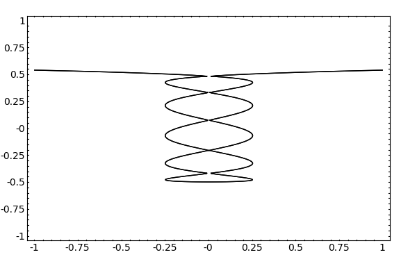
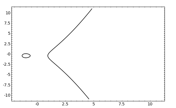
- Plotting affine and projective curves (Alex Ghitza) -- Improving the plotting usability so it is now easier to plot affine and projective curves. For example, we can plot a 5-nodal curve of degree 11:
sage: R.<x, y> = ZZ[]
sage: C = Curve(32*x^2 - 2097152*y^11 + 1441792*y^9 - 360448*y^7 + 39424*y^5 - 1760*y^3 + 22*y - 1)
sage: C.plot((x, -1, 1), (y, -1, 1), plot_points=400)
- Now we plot an elliptic curve:
sage: E = EllipticCurve('101a')
sage: C = Curve(E)
sage: C.plot()
Basic Arithmetic
- Speed-up in dividing a polynomial by an integer (William Stein, Burcin Erocal) -- Dividing a polynomial by an integer is now up to 6x faster than previously. On Debian 5.0 Lenny with kernel 2.6.24-1-686, an Intel(R) Celeron(R) CPU running at 2.00GHz with 1.0GB of RAM, one has the following timing statistics:
# BEFORE

sage: R.<x> = ZZ["x"]
sage: f = 389 * R.random_element(1000)
sage: timeit("f//389")
625 loops, best of 3: 312 µs per loop


# AFTER

sage: R.<x> = ZZ["x"]
sage: f = 389 * R.random_element(1000)
sage: timeit("f//389")
625 loops, best of 3: 48.3 µs per loop
New fast_float supports more data types with improved performance (Carl Witty) -- A rewrite of fast_float to support multiple types. Here, we get accelerated evaluation over RealField(k) as well as RDF, real double field. As compared with the previous fast_float, improved performance can range from 2% faster to more than 2x as fast. An extended list of benchmark details is available at ticket 5093.
Complex double fast callable interpreter (Robert Bradshaw) -- Support for complex double floating point (CDF). The new interpreter is implemented in the class CDFInterpreter of sage/ext/gen_interpreters.py.
Speed-up the function solve_mod() (Wilfried Huss) -- Performance improvement for the function solve_mod() is now up to 5x when solving an equation or a list of equations modulo a given integer modulus. On the machine sage.math, we have the following timing statistics:
# BEFORE

sage: x, y = var('x,y')
sage: time solve_mod([x^2 + 2 == x, x^2 + y == y^2], 14)
CPU times: user 0.01 s, sys: 0.02 s, total: 0.03 s
Wall time: 0.18 s
[(4, 2), (4, 6), (4, 9), (4, 13)]
sage:
sage: x,y,z = var('x,y,z')
sage: time solve_mod([x^5 + y^5 == z^5], 3)
CPU times: user 0.01 s, sys: 0.00 s, total: 0.01 s
Wall time: 0.10 s

[(0, 0, 0),
 (0, 1, 1),
 (0, 2, 2),
 (1, 0, 1),
 (1, 1, 2),
 (1, 2, 0),
 (2, 0, 2),
 (2, 1, 0),
 (2, 2, 1)]


# AFTER

sage: x, y = var('x,y')
sage: time solve_mod([x^2 + 2 == x, x^2 + y == y^2], 14)
CPU times: user 0.03 s, sys: 0.01 s, total: 0.04 s
Wall time: 0.16 s
[(4, 2), (4, 6), (4, 9), (4, 13)
sage:
sage: x,y,z = var('x,y,z')
sage:  time solve_mod([x^5 + y^5 == z^5], 3)
CPU times: user 0.01 s, sys: 0.01 s, total: 0.02 s
Wall time: 0.02 s

[(0, 0, 0),
 (0, 1, 1),
 (0, 2, 2),
 (1, 0, 1),
 (1, 1, 2),
 (1, 2, 0),
 (2, 0, 2),
 (2, 1, 0),
 (2, 2, 1)]
Optimized binomial function when an input is real or complex floating point (Dan Drake) -- The function binomial() for returning the binomial coefficients is now much faster. In some cases, speed efficiency can be up to 4000x. Here are some timing statistics obtained using the machine sage.math:
# BEFORE

sage: x, y = 1140000.78, 420000
sage: %timeit binomial(x, y)
10 loops, best of 3: 1.19 s per loop
sage:
sage: x, y = RR(pi^5), 10
sage: %timeit binomial(x, y)
10000 loops, best of 3: 28.2 µs per loop
sage:
sage: x, y = RR(pi^15), 500
sage: %timeit binomial(x, y)
1000 loops, best of 3: 799 µs per loop
sage:
sage: x, y = RealField(500)(1729000*sqrt(2)), 17000
sage: %timeit binomial(x, y)
10 loops, best of 3: 34.4 ms per loop


# AFTER

sage: x, y = 1140000.78, 420000
sage: %timeit binomial(x, y)
1000 loops, best of 3: 297 µs per loop
sage:
sage: x, y = RR(pi^5), 10
sage: %timeit binomial(x, y)
10000 loops, best of 3: 189 µs per loop
sage:
sage: x, y = RR(pi^15), 500
sage: %timeit binomial(x, y)
1000 loops, best of 3: 335 µs per loop
sage:
sage: x, y = RealField(500)(1729000*sqrt(2)), 17000
sage: %timeit binomial(x, y)
1000 loops, best of 3: 692 µs per loop
Enhanced nth_root() in ZZ and QQ and related utilities (John Cremona) -- Some consistency in the method nth_root() of ZZ and QQ. There are also some new utility methods for the rational numbers:
prime_to_S_part(self, S=[]) -- Returns self with all powers of all primes in S removed.
is_nth_power(self, int n) -- Returns True if self is an n-th power; else False.
is_S_integral(self, S=[]) -- Determine if the rational number is S-integral.
is_S_unit(self, S=None) -- Determine if the rational number is an S-unit.
Calculus
- Deprecate the calling of symbolic functions with unnamed arguments (Carl Witty) -- Previous releases of Sage supported symbolic functions with "no arguments". This style of constructing symbolic functions is now deprecated. For example, previously Sage allowed for defining a symbolic function in the following way
sage: x,y = var("x,y")
sage: f = x^2 + y^2
sage: f(2,3) # bad; this is deprecated
But users are encouraged to explicitly declare the variables used in a symbolic function. For instance, the following is encouraged:sage: x,y = var("x, y") sage: f(x, y) = x^2 + y^2 # this syntax is encouraged, or sage: f(2,3) # since we specified the order when defining f, we know that x=2, y=3 sage: f = x^2 + y^2 # You can also do it this way sage: f(x=2,y=3) # and then explicitly name your inputs sage: f.subs(x=2,y=3) # or use the subs "substitute" command in a similar fashion
Combinatorics
Enhancements to the Subsets and Subwords modules (Florent Hivert) -- Numerous enhancements to the modules Subsets and Subwords include:
- An implementation of subsets for finite multisets, i.e. sets with repetitions.
Adding the method __contains__ for Subsets and Subwords.
sage: S = Subsets([1, 2, 2], submultiset=True); S
SubMultiset of [1, 2, 2]
sage: S.list()
[[], [1], [2], [1, 2], [2, 2], [1, 2, 2]]
sage: Set([1,2]) in S  # this uses __contains__ in Subsets
True
sage: Set([]) in S
True
sage: Set([3]) in S
False
And here's an example of using __contains__ with Subwords:
sage: [] in Subwords([1,2,3,4,3,4,4])
True
sage: [2,3,3,4] in Subwords([1,2,3,4,3,4,4])
True
sage: [2,3,3,1] in Subwords([1,2,3,4,3,4,4])
False
- Fix and enhancements to permutations (Sebastien Labbe) -- This corrects the Robinson-Schensted algorithm on trivial permutations. It implements the inverse Robinson-Schensted algorithm:
sage: Permutation((Tableau([[1,2,4],[3]]), Tableau([[1,3,4],[2]])))
[3, 1, 2, 4]
sage: Permutation(([[1,2,4],[3]], [[1,3,4],[2]]))
[3, 1, 2, 4]
And it works for arbitrary words (with semi-standard tableaux):sage: Permutation(([[1,2,2],[3]], [[1,3,4],[2]])) [3, 1, 2, 2]
- Cleanup the interface of combinatorial classes (Florent Hivert) -- Before, the interface of combinatorial classes had two problems:
There were two redundant ways to get the number of elements len(C) and C.count(). Moreover len must return a plain int where we want an arbitrary large number and even infinity.
There were two redundant ways to get an iterator for the elements C.iterator() and iter(C) (allowing for for c in C: ...) via C.__iter__.
C.cardinality() which is more explicit and consistent with many other Sage libraries.
iter(C) / for x in C: via C.__iter__ which is clearly more Pythonic.
The functions iterator() and count() are deprecated (with a warning), but will be removed in a later release. On the other hand, there was no way to keep backward compatibility for len. Indeed, many of function such as list / filter / map try silently to call len, which would have caused myriads of warnings to be issued in seemingly unrelated places. So it was decided to simply remove it and issue an error, suggesting to call cardinality instead.
New class IntegerListLex for generating integer lists (Nicolas M. Thiery) -- The new class provides a Constant Amortized Time iterator through the combinatorial classes of integer lists. For example, we create the combinatorial class of lists of length 3 and sum 2 as follows:
sage: C = IntegerListsLex(2, length=3); C
Integer lists of sum 2 satisfying certain constraints
sage: C.count()
6
sage: [p for p in C]
[[2, 0, 0], [1, 1, 0], [1, 0, 1], [0, 2, 0], [0, 1, 1], [0, 0, 2]]
Here's the list of all compositions of 4:sage: list(IntegerListsLex(4, min_part = 1)) [[4], [3, 1], [2, 2], [2, 1, 1], [1, 3], [1, 2, 1], [1, 1, 2], [1, 1, 1, 1]]
Cleanup of crystal code (Anne Schilling) -- Cartan type is now implemented as the method cartan_type, rather than an attribute as was previously the case.
Deprecate the function RestrictedPartitions() (Dan Drake) -- The function RestrictedPartitions() in sage/combinat/partition.py is now deprecated and will be removed in a future release. Users are advised to instead consider the function Partitions() with the parts_in keyword, which is functionally equivalent to RestrictedPartitions() but is more memory and time efficient. The timing improvement in Partitions() is up to 5x faster than RestrictedPartitions(). The following memory and timing statistics are produced using the machine sage.math:
# BEFORE

sage: get_memory_usage()
721.26171875
sage: ps = RestrictedPartitions(100, ([1,6..100] + [4,9..100]))
sage: %time sum(1 for p in ps)
CPU times: user 27.26 s, sys: 1.06 s, total: 28.32 s
Wall time: 28.99 s
74040
sage: get_memory_usage()
1807.03515625

sage: get_memory_usage()
721.265625
sage: ps = RestrictedPartitions(3000, [10,50,100,500,1000])
sage: %time sum(1 for p in ps)
CPU times: user 5.60 s, sys: 0.21 s, total: 5.81 s
Wall time: 5.95 s
3506
sage: get_memory_usage()
962.54296875


# AFTER

sage: get_memory_usage()
719.3984375
sage: ps = Partitions(100, parts_in=([1,6..100] + [4,9..100]))
sage: %time sum(1 for p in ps)
CPU times: user 5.09 s, sys: 0.01 s, total: 5.10 s
Wall time: 5.10 s
74040
sage: get_memory_usage()
719.3984375

sage: get_memory_usage()
719.3984375
sage: ps = Partitions(3000, parts_in=[10,50,100,500,1000])
sage: %time sum(1 for p in ps)
CPU times: user 1.12 s, sys: 0.01 s, total: 1.13 s
Wall time: 1.13 s
3506
sage: get_memory_usage()
719.3984375
Speed-up the weyl_characters.py module (Mike Hansen, Daniel Bump) -- The timing efficiency is between 4x to 10x, depending on the operations involved. Here are some timing statistics produced using the machine sage.math:
# BEFORE

sage: R = WeylCharacterRing(['B',3], prefix = "R")
sage: %time r =  R(1,1,0)
CPU times: user 0.14 s, sys: 0.00 s, total: 0.14 s
Wall time: 0.14 s
sage:
sage: R = WeylCharacterRing(['B',3], prefix = "R")
sage: %time [R(w) for w in R.lattice().fundamental_weights()]
CPU times: user 0.25 s, sys: 0.00 s, total: 0.25 s
Wall time: 0.25 s
[R(1,0,0), R(1,1,0), R(1/2,1/2,1/2)]
sage:
sage: A2 = WeylCharacterRing(['A',2])
sage: %time [A2(0,0,0)+A2(2,1,0), A2(2,1,0)+A2(0,0,0), - A2(0,0,0)+2*A2(0,0,0),
-2*A2(0,0,0)+A2(0,0,0), -A2(2,1,0)+2*A2(2,1,0)-A2(2,1,0)]
CPU times: user 0.18 s, sys: 0.00 s, total: 0.18 s
Wall time: 0.19 s
[A2(0,0,0) + A2(2,1,0), A2(0,0,0) + A2(2,1,0), A2(0,0,0), -A2(0,0,0), 0]
sage:
sage: A2 = WeylCharacterRing(['A',2])
sage: %timeit [-x for x in [A2(0,0,0), 2*A2(0,0,0), -A2(0,0,0), -2*A2(0,0,0)]]
10 loops, best of 3: 20 ms per loop
sage:
sage: A2 = WeylCharacterRing(['A',2])
sage: chi = A2(0,0,0)+2*A2(1,0,0)+3*A2(2,0,0)
sage: mu =  3*A2(0,0,0)+2*A2(1,0,0)+A2(2,0,0)
sage: %timeit chi - mu
100 loops, best of 3: 8.16 ms per loop
sage:
sage: A2 = WeylCharacterRing(['A',2])
sage: chi = A2(1,0,0)
sage: %time [chi^k for k in range(6)]
CPU times: user 1.05 s, sys: 0.02 s, total: 1.07 s
Wall time: 1.07 s

[A2(0,0,0),
 A2(1,0,0),
 A2(1,1,0) + A2(2,0,0),
 A2(1,1,1) + 2*A2(2,1,0) + A2(3,0,0),
 3*A2(2,1,1) + 2*A2(2,2,0) + 3*A2(3,1,0) + A2(4,0,0),
 5*A2(2,2,1) + 6*A2(3,1,1) + 5*A2(3,2,0) + 4*A2(4,1,0) + A2(5,0,0)]


# AFTER

sage: R = WeylCharacterRing(['B',3], prefix = "R")
sage: %time r =  R(1,1,0)
CPU times: user 0.03 s, sys: 0.00 s, total: 0.03 s
Wall time: 0.03 s
sage:
sage: R = WeylCharacterRing(['B',3], prefix = "R")
sage: %time [R(w) for w in R.lattice().fundamental_weights()]
CPU times: user 0.05 s, sys: 0.00 s, total: 0.05 s
Wall time: 0.05 s
[R(1,0,0), R(1,1,0), R(1/2,1/2,1/2)]
sage:
sage: A2 = WeylCharacterRing(['A',2])
sage: %time [A2(0,0,0)+A2(2,1,0), A2(2,1,0)+A2(0,0,0), - A2(0,0,0)+2*A2(0,0,0), -2*A2(0,0,0)+A2(0,0,0), -A2(2,1,0)+2*A2(2,1,0)-A2(2,1,0)]
CPU times: user 0.04 s, sys: 0.00 s, total: 0.04 s
Wall time: 0.04 s
[A2(0,0,0) + A2(2,1,0), A2(0,0,0) + A2(2,1,0), A2(0,0,0), -A2(0,0,0), 0]
sage:
sage: A2 = WeylCharacterRing(['A',2])
sage: %timeit [-x for x in [A2(0,0,0), 2*A2(0,0,0), -A2(0,0,0), -2*A2(0,0,0)]]
100 loops, best of 3: 3.33 ms per loop
sage:
sage: A2 = WeylCharacterRing(['A',2])
sage: chi = A2(0,0,0)+2*A2(1,0,0)+3*A2(2,0,0)
sage: mu =  3*A2(0,0,0)+2*A2(1,0,0)+A2(2,0,0)
sage: %timeit chi - mu
1000 loops, best of 3: 771 µs per loop
sage:
sage: A2 = WeylCharacterRing(['A',2])
sage: chi = A2(1,0,0)
sage: %time [chi^k for k in range(6)]
CPU times: user 0.20 s, sys: 0.00 s, total: 0.20 s
Wall time: 0.20 s

[A2(0,0,0),
 A2(1,0,0),
 A2(1,1,0) + A2(2,0,0),
 A2(1,1,1) + 2*A2(2,1,0) + A2(3,0,0),
 3*A2(2,1,1) + 2*A2(2,2,0) + 3*A2(3,1,0) + A2(4,0,0),
 5*A2(2,2,1) + 6*A2(3,1,1) + 5*A2(3,2,0) + 4*A2(4,1,0) + A2(5,0,0)]
Commutative Algebra
New function weil_restriction() on multivariate ideals (Martin Albrecht) -- The new function weil_restriction() computes the Weil restriction of a multivariate ideal over some extension field. A Weil restriction is also known as a restriction of scalars. Here's an example on computing a Weil restriction:
sage: k.<a> = GF(2^2)
sage: P.<x,y> = PolynomialRing(k, 2)
sage: I = Ideal([x*y + 1, a*x + 1])
sage: I.variety()
[{y: a, x: a + 1}]
sage: J = I.weil_restriction()
sage: J
Ideal (x1*y0 + x0*y1 + x1*y1, x0*y0 + x1*y1 + 1, x0 + x1, x1 + 1) of
Multivariate Polynomial Ring in x0, x1, y0, y1 over Finite Field of size 2
Varieties and polynomial ideals (John Perry) -- Support for polynomial ideals over finite fields of characteristics greater than what Singular supports. Thus in case where the characteristic of the base field is too large for Singular, we use a toy implementation to compute the variety of the polynomial ideal. This implementation is contained in the new module /sage/rings/polynomial/toy_variety.py, which implements an educational version of the Groebner basis algorithm.
Extended Euclidean algorithm for polynomials over GF(2) (Mike Hansen) -- An xgcd() method for polynomials with base field being the Galois field of 2 elements.
New method apply_morphism() for ideals (Nick Alexander) -- The new method apply_morphism() in sage/rings/ideal.py applies a specified morphism to every element of an ideal.
Doctest
New and improved random testing module (Carl Witty) -- The new and improved random tester can be found in sage/misc/random_testing.py. The random testing module is useful for Sage modules that do random testing in their doctests by constructing test cases using a random number generator. It provides a decorator to help write random testers that meet the following goals:
- To get the broadest possible test coverage by using different random seeds in doctests.
- To be able to reproduce problems when debugging.
Geometry
Improved enumeration of vertices and 0-dimensional faces of LatticePolytope objects (Andrey Novoseltsev) -- There was an inconsistency between indicies of vertices, i.e. columns of the .vertices() matrix, and indicies of 0-dimensional faces, i.e. objects returned by .faces(dim=0). For example, the 5-th 0-dimensional face could be generated by the 7-th vertex, etc. Now the i-th 0-dimensional face is generated by the i-th vertex. (The reason for the old behaviour was the output of the underlying software package PALP, now there is extra sorting.)
Graph Theory
Improved time efficiency of all_graph_colorings() function (Carlo Hamalainen) -- The function all_graph_colorings() in sage/graphs/graph_coloring.py now uses the C++ dancing links implementation instead of the Cython implementation in computing graph colorings. In some cases, the speed-up can be up to 5x. Here are some timing statistics obtained using the machine sage.math. First, define a testing script called color_test.sage with the following content:
from sage.graphs.graph_coloring import all_graph_colorings
set_random_seed(0)
def foo():
    G = graphs.RandomGNP(10, 0.5)
    chrom = G.chromatic_number()
    n = 0
    for C in all_graph_colorings(G, chrom):
        parts = [C[k] for k in C]
        for P in parts:
            l = len(P)
            for i in range(l):
                for j in range(i+1,l):
                    if G.has_edge(P[i],P[j]):
                        raise RuntimeError, "Coloring Failed."
        n+=1
    print "G has %s 3-colorings."%n
timeit("foo()")
Next, we run tests as follows:# BEFORE [mvngu@sage mvngu]$ sage-3.4-sage.math-only-x86_64-Linux/sage color_test.sage 5 loops, best of 3: 65.8 ms per loop [mvngu@sage mvngu]$ sage-3.4-sage.math-only-x86_64-Linux/sage color_test.sage 5 loops, best of 3: 64.4 ms per loop [mvngu@sage mvngu]$ sage-3.4-sage.math-only-x86_64-Linux/sage color_test.sage 5 loops, best of 3: 64.2 ms per loop # AFTER [mvngu@sage mvngu]$ sage-3.4.1-sage.math-only-x86_64-Linux/sage color_test.sage 5 loops, best of 3: 14.2 ms per loop [mvngu@sage mvngu]$ sage-3.4.1-sage.math-only-x86_64-Linux/sage color_test.sage 5 loops, best of 3: 14.4 ms per loop [mvngu@sage mvngu]$ sage-3.4.1-sage.math-only-x86_64-Linux/sage color_test.sage 5 loops, best of 3: 14.3 ms per loop
Graphics
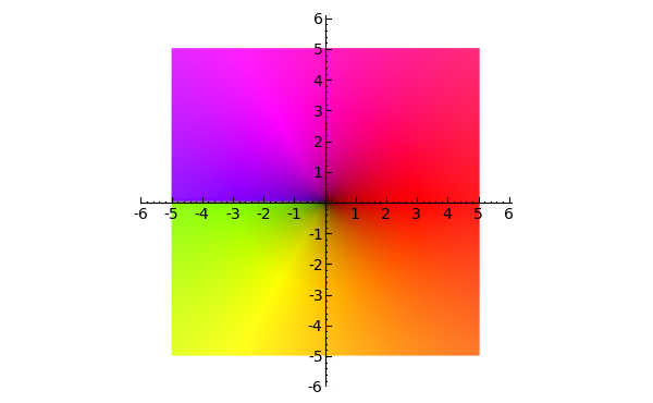
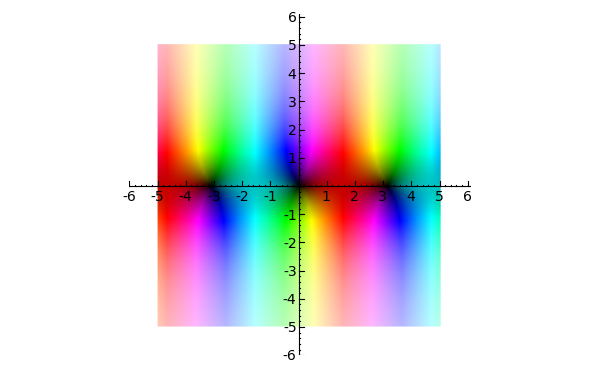
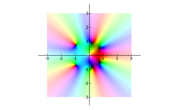
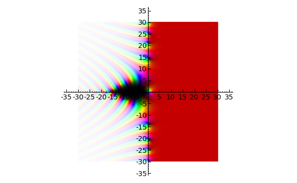
Color complex plotting (Robert Bradshaw) -- New function complex_plot() for plotting functions of a complex variable. The function complex_plot() takes a complex function f(z) of one variable and plots output of the function over the specified xrange and yrange. The magnitude of the output is indicated by the brightness (with zero being black and infinity being white), while the argument is represented by the hue with red being positive real and increasing through orange, yellow, etc. as the argument increases. The general syntax of the function is complex_plot(f, (xmin, xmax), (ymin, ymax), ...). The following code produces a plot of the square root function:
sage: complex_plot(sqrt, (-5, 5), (-5, 5))
- Here's a plot of the sine function:
sage: complex_plot(sin, (-5, 5), (-5, 5))
- Plot of a meromorphic with some nice zeros and a pole:
sage: f(z) = z^5 + z - 1 + 1/z
sage: complex_plot(f, (-3, 3), (-3, 3))
- A plot of the Riemann zeta function:
sage: complex_plot(zeta, (-30,30), (-30,30))
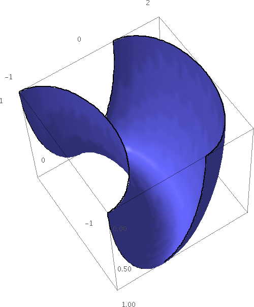
Parameter boundary_style for parametric 3-D plots (Bill Cauchois) -- Implement boundary_style parameter to describe how to draw the boundaries of regions by giving options that are passed to the line3d command. Here's an example:
sage: u, v = var("u, v")
sage: parametric_plot3d((cos(u), sin(u) + cos(v), sin(v)), (u,0,pi), (v,0,pi), boundary_style={"color":"black", "thickness":2}, zoom=1.2)
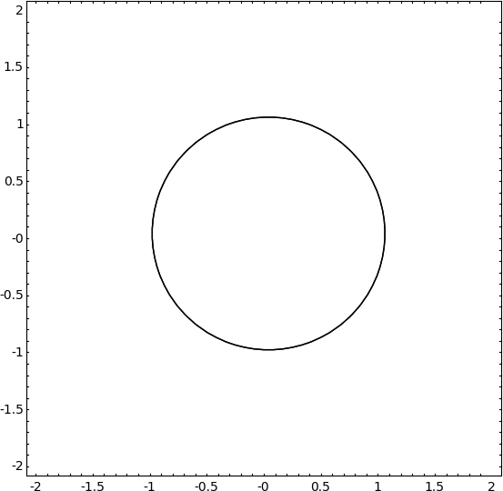
Support implicit plotting of equations (William Stein) -- The function implicit_plot now supports implicit plotting of equations. Here's an example implicit plot of the unit circle:
sage: x, y = var("x, y ")
sage: implicit_plot(x^2 + y^2 == 1, (x,-2,2), (y,-2,2)).show(aspect_ratio=1)
Group Theory
- Speed-up in comparing elements of a permutation group (John Palmieri, Robert Bradshaw) -- For elements of a permutation group, comparison between those elements is now up to 13x faster. On Mac OS X 10.4 with Intel Core 2 duo running at 2.33 GHz, one has the following improvement in timing statistics:
# BEFORE sage: a = SymmetricGroup(20).random_element() sage: b = SymmetricGroup(10).random_element() sage: timeit("a == b") 625 loops, best of 3: 3.19 µs per loop # AFTER sage: a = SymmetricGroup(20).random_element() sage: b = SymmetricGroup(10).random_element() sage: time v = [a == b for _ in xrange(2000)] CPU times: user 0.00 s, sys: 0.00 s, total: 0.00 s Wall time: 0.00 s sage: timeit("a == b") 625 loops, best of 3: 240 ns per loop - Optimize small permutation group elements (Robert Bradshaw) -- Avoid allocation for very small permutation group elements, otherwise there can be a significant cost of element creation. In some cases, there can be up to 17% efficiency. The following timing statistics were obtained using the machine sage.math:
# BEFORE

sage: G = SymmetricGroup(3)
sage: L = [G.random_element() for _ in range(100)] * 17
sage: %timeit prod(L)
1000 loops, best of 3: 290 µs per loop
sage:
sage: G = SymmetricGroup(10)
sage: L = [G.random_element() for _ in range(100)] * 17
sage: %timeit prod(L)
1000 loops, best of 3: 321 µs per loop


# AFTER

sage: G = SymmetricGroup(3)
sage: L = [G.random_element() for _ in range(100)] * 17
sage: %timeit prod(L)
1000 loops, best of 3: 240 µs per loop
sage:
sage: G = SymmetricGroup(10)
sage: L = [G.random_element() for _ in range(100)] * 17
sage: %timeit prod(L)
1000 loops, best of 3: 271 µs per loop
Linear Algebra
Deprecate the function invert() (John H. Palmieri) -- The function invert() for calculating the inverse of a dense matrix with rational entries is now deprecated. Instead, users are now advised to use the function inverse(). Here's an example of using the function inverse():
sage: a = matrix(QQ, 2, [1, 5, 17, 3])
sage: a.inverse()
[-3/82  5/82]
[17/82 -1/82]
Speed-up in calculating determinants of matrices (John H. Palmieri) -- For matrices over Z/nZ with n composite, calculating their determinants is now up to 1500x faster. On Debian 5.0 Lenny with kernel 2.6.24-1-686, an Intel(R) Celeron(R) 2.00GHz CPU with 1.0GB of RAM, one has the following timing statistics:
# BEFORE

sage: time random_matrix(Integers(26), 10).determinant()
CPU times: user 15.52 s, sys: 0.02 s, total: 15.54 s
Wall time: 15.54 s
13
sage: time random_matrix(Integers(256), 10).determinant()
CPU times: user 15.38 s, sys: 0.00 s, total: 15.38 s
Wall time: 15.38 s
144


# AFTER

sage: time random_matrix(Integers(26), 10).determinant()
CPU times: user 0.01 s, sys: 0.00 s, total: 0.01 s
Wall time: 0.01 s
23
sage: time random_matrix(Integers(256), 10).determinant()
CPU times: user 0.00 s, sys: 0.00 s, total: 0.00 s
Wall time: 0.00 s
Optimize string representation for matrices over GF(2) (Robert Bradshaw) -- Optimize the method str() for returning a string representation of a matrix over the field GF(2). The efficiency gain is up to 26x. The following timing statistics were obtained using the machine sage.math:
# BEFORE

sage: a = random_matrix(GF(2),1000)
sage: %time b = a.str()
CPU times: user 0.25 s, sys: 0.01 s, total: 0.26 s
Wall time: 0.26 s


# AFTER
sage: a = random_matrix(GF(2),1000)
sage: %time b = a.str()
CPU times: user 0.00 s, sys: 0.01 s, total: 0.01 s
Wall time: 0.01 s
- Inverse operation for matrices over non-integral domain (William Stein) -- Inverse operation for matrices over the integers modulo a composite modulus. Here are some examples for working such matrices:
sage: m = matrix(Zmod(49), 2, [2,1,3,3])
sage: type(m)
<type 'sage.matrix.matrix_modn_dense.Matrix_modn_dense'>
sage: m.inverse()

[ 1 16]
[48 17]
sage: m = matrix(Zmod(2^100), 2, [2,1,3,3])
sage: type(m)
<type 'sage.matrix.matrix_generic_dense.Matrix_generic_dense'>
sage: m.inverse() * m

[1 0]
[0 1]
sage: m.inverse()

[                              1  422550200076076467165567735125]
[1267650600228229401496703205375  422550200076076467165567735126]
Miscellaneous
Deprecate function jsmath() from the command line (John H. Palmieri) -- The function jsmath() is now deprecated and will be removed from a future release. Users are advised to consider the function html() instead. For example, users should replace jsmath("MATH", mode="display") with html("$$MATH$$"), and replace jsmath("MATH", mode="inline") with html("$MATH$").
Modular Forms
Implement Pizer's algorithm for computing Brandt Modules and Brandt Matrices (William Stein, Gonzalo Tornaria, Jon Bober, Alia Hamieh, Victoria de Quehen) -- The new module sage/modular/quatalg/brandt.py implements the algorithm of Pizer for computing modular forms using quaternion algebras. See the sage wiki for more information on this implementation and Pizer's original algorithm.
sage: B = BrandtModule(11,15)
sage: B.hecke_matrix(2).charpoly().factor()
(x - 3) * (x - 1)^4 * (x + 2)^4 * (x^2 - 3) * (x^2 + 2*x - 1) * (x^2 - 2*x - 1)^2 * (x^3 + x^2 - 5*x - 1)
sage: B.right_ideals()
(Fractional ideal (2 + 2*j, 2*i + 46*k, 4*j, 60*k), Fractional ideal (2 + 2*j + 60*k, 2*i + 4*j + 46*k, 8*j, 120*k), ... Fractional ideal (2 + 2*i + 10*j + 226*k, 4*i + 12*j + 152*k, 16*j + 240*k, 480*k))
This gives the first ever open source implementation of computation of Tamagawa numbers of (certain) modular abelian varieties:sage: A = J0(55)[3]; A Simple abelian subvariety 55b(1,55) of dimension 2 of J0(55) sage: A.dimension() 2 sage: A.tamagawa_number(5) 2 sage: A.tamagawa_number(11) 2
Multiplication for modular forms (David Loeffler) -- New method __mul__ for ModularFormElement objects, which essentially allows for multiplication of modular forms. Here's an example with character:
sage: f = ModularForms(DirichletGroup(3).0, 3).0
sage: f * f
1 + 108*q^2 + 144*q^3 + 2916*q^4 + 8640*q^5 + O(q^6)
sage: (f*f).parent()
Modular Forms space of dimension 3 for Congruence Subgroup Gamma0(3) of weight 6 over Rational Field
sage: (f*f*f).parent()
Modular Forms space of dimension 4, character [-1] and weight 9 over Rational Field
And here's an example without:sage: f = ModularForms(Gamma1(3), 5).0 sage: f*f 1 - 180*q^2 - 480*q^3 + 8100*q^4 + 35712*q^5 + O(q^6) sage: (f*f).parent() Modular Forms space of dimension 4 for Congruence Subgroup Gamma1(3) of weight 10 over Rational Field
Improvements to congruence subgroups (David Loeffler, Chris Kurth) -- The code for congruence subgroups is now split up into several files under sage/modular/arithgroup. The previous file sage/modular/congroup.py still exists, so pickles created with previous versions should unpickle safely under the new one. New functionality includes:
Handling arbitrary (not necessarily congruence) finite index subgroups of SL2(Z), defined in terms of the right permutation action of SL2(Z) on their cosets. This is based on code from Chris Kurth's KFarey package.
A variety of tools for calculating quantities relating to the geometry of the modular curve X(Gamma) for arbitrary Gamma, including finding the genus, the set of cusps with their widths and their regularity, and the dimensions of their modular forms spaces for all weights other than 1.
- Overconvergent modular forms (David Loeffler) -- The space of overconvergent modular forms is in some sense a "p-adic completion" of the space of classical modular forms, which is important in understanding congruence properties of modular forms. This version of Sage incorporates an algorithm (based on work of Smithline, Buzzard and Calegari, and others) which calculates the matrices of Hecke operators on these spaces and approximations to the q-expansions of eigenforms, for certain small levels and primes (but any weight).
Notebook
- Unicode support for the Sage Notebook (Mike Hansen, Dan Drake).
Worksheets open in new page/tab (William Stein, John Palmieri) -- When one opens a worksheet, it appears in a new tab (or window) so that there is no history, hence nothing to accidentally go back to. The "new worksheet" button would also open a new worksheet in a new tab. Note that with this new feature, there's still a known issue. If one opens up a worksheet, work for a while with that worksheet, then hit "Save & Quit" or "Discard & Quit", one would now have two tabs open listing the active worksheets.
Number Theory
Improve efficiency of multiplicative_order() for number field elements (John Cremona) -- Before, the following example
sage: x = polygen(QQ)
sage: K.<a>=NumberField(x^40 - x^20 + 4)
sage: u = 1/4*a^30 + 1/4*a^10 + 1/2
sage: u.multiplicative_order()
6
sage: a.multiplicative_order()
+Infinity
would have required raising a to the power 2**40. Furthermore, previously the following example
sage: K.<a, b> = NumberField([x^2 + x + 1, x^2 - 3])
sage: z = (a - 1)*b/3
sage: z.multiplicative_order()
+Infinity
returns +Infinity, which is wrong. This is now fixed, as illustrated here:
sage: K.<a, b> = NumberField([x^2 + x + 1, x^2 - 3])
sage: z = (a - 1)*b/3
sage: z.multiplicative_order()
12
New functionalities for relative number fields (Francis Clarke) -- Many improvements for relative number fields. In particular a whole load of previously unimplemented functions for ideals in a relative number field now work, and others work better. For several functions, the distinction between the relative and absolute version has been made explicit in order to avoid ambiguity. Thus, for example, for a relative number field both relative_degree and absolute_degree are defined but degree is unimplemented, while for an absolute number field relative_degree, absolute_degree and degree are all defined (with the same meaning).
- Wrapper for hyperelliptic curve zeta functions (David Harvey, Nick Alexander) -- This is a basic wrapper. Here's an example on using it:
sage: R.<x> = PolynomialRing(GF(10007))
sage: H = HyperellipticCurve(x^7 + x + 1)
sage: H.frobenius_polynomial()
x^6 + 4*x^5 + 21884*x^4 - 99088*x^3 + 218993188*x^2 + 400560196*x + 1002101470343
- Quadratic twists for p-adic L-functions (Chris Wuthrich) -- New features for computing p-adic L-function of quadratic twists of elliptic curves.
Unifying the computation of Galois groups (David Loeffler) -- One can now compute the Galois group of a number field using the function galois_group(), which by default calls Pari.
New functions for computing Hilbert class polynomials (Eduardo Ocampo Alvarez, Andrey Timofeev, Alex Ghitza) -- The new method hilbert_class_polynomial() allows for Computing the Hilbert class polynomial of a quadratic field. Currently, there's only support for imaginary quadratic fields.
Support for Kloosterman sums (Kilian Kilger) -- Adds support for exact and numerical evaluation of "twisted" Kloosterman sums. This generalizes Gauss sums, Salie sums and normal Kloosterman sums. The method kloosterman_sum() returns the "twisted" Kloosterman sum associated to a Dirichlet character. The method kloosterman_sum_numerical() returns the Kloosterman sum associated to a Dirichlet character as an approximate complex number with a specified number of bits of precision.
- Exposes Pari's galois and finer number field interfaces (Nick Alexander) -- New functions for interfacing with Pari's galois computation functionalities include:
nfgaloisconj(self) -- Returns a list of conjugates of a root.
nfroots(self, poly) -- Returns the roots of poly in the number field self without multiplicity.
automorphisms(self) -- Computes all Galois automorphisms of self.
Enhanced handling of elliptic curve twists (John Cremona) -- New methods is_quadratic_twist(), is_quartic_twist(), is_sextic_twist() for detecting twists between curves (and returning the appropriate twisting parameter). The EllipticCurve(j) constructor is now deprecated and will be removed in a future release. Users are advised to consider the constructor EllipticCurve_from_j(j) instead. Over the rationals, the constructor EllipticCurve_from_j(j) gives the minimal twist, i.e. a curve with the correct j and minimal conductor.
Conjectural (analytic) order of Sha for elliptic curves over Heegner quadratic imaginary fields (William Stein) -- New method heegner_sha_an() for computing the conjectural (analytic) order of Sha. In computing this analytic order of Sha, we assume a default 53-bit of precision, but the exact number of precision can be changed using the argument prec. The new method can be found in sage/schemes/elliptic_curves/ell_rational_field.py.
Number field ideal utilities (Maite Aranes) -- Various new functions in sage/libs/pari/gen.pyx and sage/rings/number_field/number_field_ideal.py for working with ideals in number fields. These include:
New method nfeltreduce(self, x, I) -- Given an ideal I in Hermite normal form and an element x of the pari number field self, find an element r in self such that x - r belongs to the ideal and r is small.
New method invertible_residues_mod_units(self, units=[], reduce=True) -- Returns an iterator through a list of invertible residues modulo this integral ideal and modulo the group generated by the given units.
New method idealcoprime(self, J) -- Returns l such that l * self is coprime to J.
New method small_residue(self, f) -- Given an element f of the ambient number field, return an element g such that f - g belongs to the ideal self (which must be integral), and g is small.
New method idealstar(self, flag=1) -- Returns the finite abelian group (O_K/I)^*, where I is the ideal self of the number field K and O_K is the ring of integers of K.
New method ideallog(self, x) -- Returns the discrete logarithm of x with respect to the generators given in the bid structure of the ideal self.
Enhanced support for number field unit groups (John Cremona) -- New class UnitGroup in the module sage/rings/number_field/unit_group.py for representing the unit group of a number field. As before, the units are computed using the Pari library, but now it is easier (for example) to obtain all generators of the unit group. Also, there's a wrapping for the Pari function bnfisunit() which implements a discrete log function to express any unit in terms of the generators.
Packages
Upgrade to Cython version 0.11 upstream release (Robert Bradshaw) -- Based on Pyrex, Cython is a language that closely resembles Python and developed for writing C extensions for Python. For critical functionalities and performance, Sage uses Cython to generate very efficient C code from Cython code, for wrapping external C libraries, and for fast C modules that speed up the execution of Python code.
Upgrade MPIR to version 1.1 upstream release (Michael Abshoff) -- MPIR is a library for multiprecision integers and rationals based on the GMP project. Among other things, MPIR aims to provide native build capability under Windows.
Upgrade FLINT to version 1.2.4 upstream release (Burcin Erocal) -- FLINT (Fast Library for Number Theory) is a library for univariate polynomial arithmetic over Z/nZ.
Upgrade libpng to version 1.2.35 upstream release (Michael Abshoff) -- Version 1.2.35 fixes a number of security issues, which are documented at the libpng project web site.
Upgrade Clisp to version 2.47 latest upstream release (Gonzalo Tornaria, Michael Abshoff) -- The new package clisp-2.47.p0.spkg also introduces noreadline mode dynamically for Clisp and Maxima.
Upgrade SymPy to version 0.6.4 latest upstream release (Ondrej Certik) -- SymPy is a Python library for symbolic mathematics.
Downgrade GAP from version 4.4.12 down to version 4.4.10 (Michael Abshoff) -- The previous package gap-4.4.12.p1.spkg didn't work smoothly under Itanium processors. Moreover, there was a reported problem with the function deepcopy() when used with WeylGroup. See this sage-devel thread for further details.
Update to optional package kash3-2008-07-31.spkg (William Stein) -- Kash is a computer algebra system for computations in algebraic number theory. Kash is closed source, but binaries are freely available.
Experimental package ets-3.1.1.rev23241.spkg, also including Chaco and Mayavi2 (Jaap Spies) -- The Enthought Tool Suite is a collection of components that comprises 2-D and 3-D graphics, scientific, mathematics and development libraries.
Improvement to experimental package vtk-5.2.1.spkg (Jaap Spies) -- The Visualization Toolkit (VTK) is an open-source, freely available software system for 3-D computer graphics, image processing, and visualization. VTK consists of a C++ class library and several interpreted interface layers including Tcl/Tk, Java, and Python.
Symbolics
- Pynac interface improvements (Burcin Erocal) -- Some enhancements to the Pynac interface and two new methods:
find(self, pattern) -- Find all occurrences of the given pattern in this expression. Note that once a subexpression matches the pattern, the search doesn't extend to subexpressions of it.
is_polynomial(self, var) -- Returns True if self is a polynomial in the given variable.
Topology
Implements simplicial complexes, chain complexes, and their homology (John Palmieri) -- Simplicial complexes are implemented in the new module sage/homology/simplicial_complex.py, and chain complexes are implemented in the new module sage/homology/chain_complex.py. Here's an example on using the new class SimplicialComplex and the method homology():
sage: circle = SimplicialComplex(2, [[0,1], [1,2], [2,0]])
sage: circle.homology(0)  # 'homology' means reduced homology
0
sage: circle.homology(1, base_ring=QQ)  # homology with coefficients
Vector space of dimension 1 over Rational Field
A number of simplicial complexes are already defined. For example, type simplicial_complexes. and then hit the TAB key to get a list.
sage: K = simplicial_complexes.KleinBottle()
sage: K.cohomology()  # without an argument, get all homology groups as a dictionary
{0: 0, 1: Z, 2: C2}
sage: S = simplicial_complexes.NotIConnectedGraphs(6,2)  # an example from graph theory
sage: S.f_vector()
[1, 15, 105, 455, 1365, 3003, 4945, 5715, 3990, 1470, 306, 30]
sage: sum(S.f_vector())  # total number of simplices
21400
sage: time S.homology()  # on a 2.4 GHz iMac
Wall time: 20.31 s
{0: 0, 1: 0, 2: 0, 3: 0, 4: 0, 5: 0, 6: 0, 7: Z^24, 8: 0, 9: 0, 10: 0}
Each simplicial complex has an associated chain complex, and chain complexes can also be defined on their own:sage: S = simplicial_complexes.NotIConnectedGraphs(6,2) sage: C = S.chain_complex() sage: C.differential() {0: [], 1: 15 x 105 sparse matrix over Integer Ring, 2: 105 x 455 sparse matrix over Integer Ring, 3: 455 x 1365 sparse matrix over Integer Ring, 4: 1365 x 3003 sparse matrix over Integer Ring, 5: 3003 x 4945 sparse matrix over Integer Ring, 6: 4945 x 5715 sparse matrix over Integer Ring, 7: 5715 x 3990 sparse matrix over Integer Ring, 8: 3990 x 1470 sparse matrix over Integer Ring, 9: 1470 x 306 sparse matrix over Integer Ring, 10: 306 x 30 sparse matrix over Integer Ring} sage: D = ChainComplex([identity_matrix(2), matrix(3,2), identity_matrix(3)]) sage: D Chain complex with at most 4 nonzero terms over Integer Ring. sage: D.differential(0) [1 0] [0 1] sage: D.differential(1) [0 0] [0 0] [0 0] sage: D.differential(2) [1 0 0] [0 1 0] [0 0 1] sage: D.differential(3) []
