|
Size: 1009
Comment: started describing timing tests
|
← Revision 7 as of 2008-11-14 13:41:55 ⇥
Size: 3317
Comment: converted to 1.6 markup
|
| Deletions are marked like this. | Additions are marked like this. |
| Line 5: | Line 5: |
| (TBA) | Interestingly, for every pair of systems, there are ranges of degrees and coefficient sizes where either system can win. The following three graphs show the results. * The horizontal axis is the base-10 logarithm of the polynomial degree. (So 4 means degree 10000.) * The vertical axis is the base-10 logarithm of the number of bits in the coefficients. (So 4 means 10000-bit coefficients.) * The colour of the circles show the ''relative'' times. MAGMA is red, NTL is blue, PARI is green. For example, a large red circle means that MAGMA was ''fast'' compared to the other system on that graph. The size of the circle indicates how much faster: the area of the circle is proportional to the logarithm of the ratio between the two times. The ratio is cropped at 10, so the graphs don't distinguish between being 10 times faster or being 1000 times faster. ==== MAGMA vs NTL: ==== {{attachment:magma_vs_ntl.png}} ==== MAGMA vs PARI: ==== {{attachment:magma_vs_pari.png}} ==== PARI vs NTL: ==== {{attachment:pari_vs_ntl.png}} |
| Line 9: | Line 27: |
| (TBA) | * [[attachment:output.txt]] This is the file produced by poly_multiply_benchmark.sage. The fields in each line are: * the polynomial degree * the number of bits in each coefficient (e.g. if it's 8 then the coefficients are between -256 and 256) * which system is being tested * the average time over the five samples (see "methodology" below) * the difference between the maximum time and the minimum time of the five samples * the number of trial multiplications used in each sample |
| Line 13: | Line 42: |
| (TBA) | * [[attachment:poly_multiply_benchmark.sage]] (runs the timing tests) * [[attachment:make_graphs.sage]] (generates the pretty graphs) |
| Line 19: | Line 49: |
| 1. Generate a random pair of polynomials and import it into the system. | * Generate a random pair of polynomials and import it into the system. |
| Line 21: | Line 51: |
| 2. Try multiplying once, see how long that takes. If that took less than half a second, try multiplying twice, see how long that takes. Keep doubling the number of trials until we find some N such that N trials take at least half a second. | * Try multiplying once, see how long that takes. If that took less than half a second, try multiplying twice, see how long that takes. Keep doubling the number of trials until we find some N such that N trials take at least half a second. |
| Line 23: | Line 53: |
| 3. Time N trials. Divide the answer by N to find out how long each trial took. Do this five times. Report the average of the five samples, and also report the difference between the maximum and minimum (just to make sure we're not being led totally astray by irregularities). | * Time N trials. Divide the answer by N to find out how long each trial took. Do this five times. Report the average of the five samples, and also report the difference between the maximum and minimum (just to make sure we're not being led totally astray by irregularities). === Problems with the methodology === * For the very fast operations (e.g. when the degree is very small), it's not clear how much overhead is being incurred by the python interpreter. So I'm not sure how much of the time is really being spent on the multiplication. * Update: I did some further tests using NTL directly from C++, and in some of the small cases (where the above graphs show NTL at the greatest disadvantage) it was faster than the above tests indicate by a factor of about 2. So basically our NTL wrapper really sucks for small polynomials. But still it was several times slower than MAGMA in that range. |
This page describes some timing tests I did to compare the speed of polynomial multiplication over Z for MAGMA, NTL and PARI. The timings were performed on sage.math.washington.edu.
Summary of results
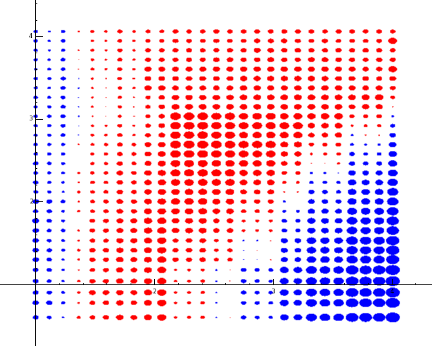
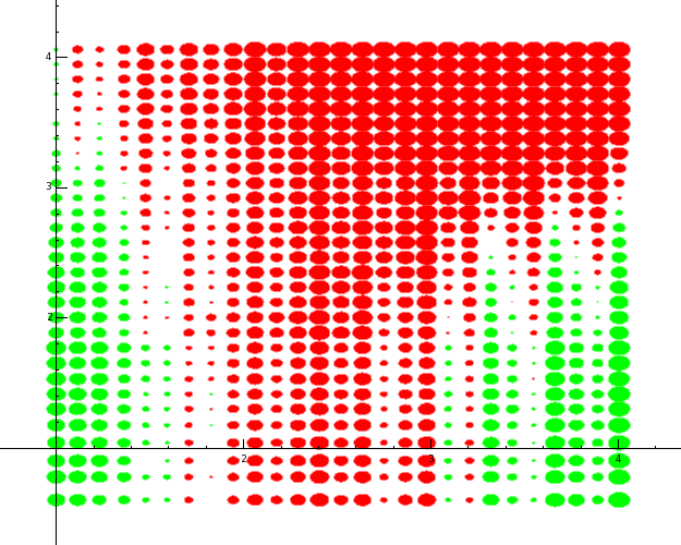
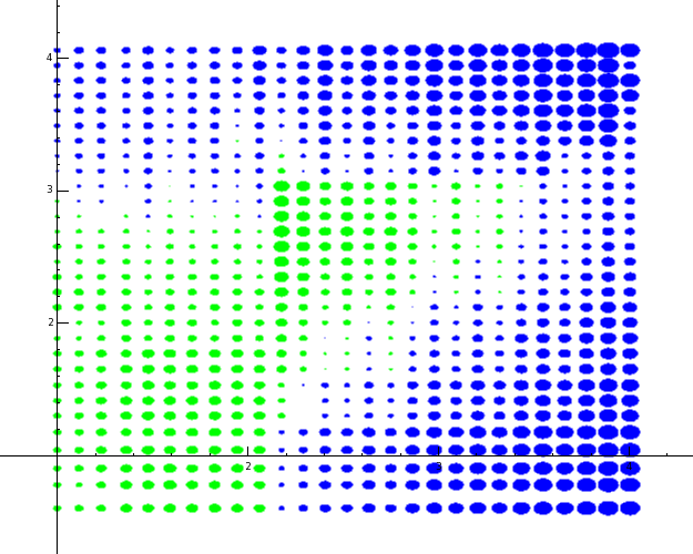
Interestingly, for every pair of systems, there are ranges of degrees and coefficient sizes where either system can win.
The following three graphs show the results.
- The horizontal axis is the base-10 logarithm of the polynomial degree. (So 4 means degree 10000.)
- The vertical axis is the base-10 logarithm of the number of bits in the coefficients. (So 4 means 10000-bit coefficients.)
The colour of the circles show the relative times. MAGMA is red, NTL is blue, PARI is green. For example, a large red circle means that MAGMA was fast compared to the other system on that graph. The size of the circle indicates how much faster: the area of the circle is proportional to the logarithm of the ratio between the two times. The ratio is cropped at 10, so the graphs don't distinguish between being 10 times faster or being 1000 times faster.
MAGMA vs NTL:

MAGMA vs PARI:

PARI vs NTL:

Raw output data
This is the file produced by poly_multiply_benchmark.sage.
The fields in each line are:
- the polynomial degree
- the number of bits in each coefficient (e.g. if it's 8 then the coefficients are between -256 and 256)
- which system is being tested
- the average time over the five samples (see "methodology" below)
- the difference between the maximum time and the minimum time of the five samples
- the number of trial multiplications used in each sample
The code
poly_multiply_benchmark.sage (runs the timing tests)
make_graphs.sage (generates the pretty graphs)
Methodology
For each pair of degree and coefficient size, and for each system (MAGMA, PARI, NTL), I did the following:
- Generate a random pair of polynomials and import it into the system.
- Try multiplying once, see how long that takes. If that took less than half a second, try multiplying twice, see how long that takes. Keep doubling the number of trials until we find some N such that N trials take at least half a second.
- Time N trials. Divide the answer by N to find out how long each trial took. Do this five times. Report the average of the five samples, and also report the difference between the maximum and minimum (just to make sure we're not being led totally astray by irregularities).
Problems with the methodology
- For the very fast operations (e.g. when the degree is very small), it's not clear how much overhead is being incurred by the python interpreter. So I'm not sure how much of the time is really being spent on the multiplication.
- Update: I did some further tests using NTL directly from C++, and in some of the small cases (where the above graphs show NTL at the greatest disadvantage) it was faster than the above tests indicate by a factor of about 2. So basically our NTL wrapper really sucks for small polynomials. But still it was several times slower than MAGMA in that range.
