|
Size: 13579
Comment: Summarize #5557, #5381, #4337
|
Size: 13794
Comment: More reminders to showcase features
|
| Deletions are marked like this. | Additions are marked like this. |
| Line 42: | Line 42: |
| * FIXME: summarize #5582 |
|
| Line 67: | Line 70: |
* FIXME: summarize #5879 |
|
| Line 143: | Line 149: |
| * FIXME: summarize #6077 * FIXME: summarize #5581 |
|
| Line 170: | Line 181: |
| Line 171: | Line 183: |
* FIXME: summarize #4875 |
|
| Line 331: | Line 346: |
* FIXME: summarize #5120 |
|
| Line 412: | Line 430: |
| * FIXME: summarize #5930 |
Sage 4.0 Release Tour
Sage 4.0 was released on FIXME. For the official, comprehensive release note, please refer to sage-4.0.txt. A nicely formatted version of this release tour can be found at FIXME. The following points are some of the foci of this release:
Algebra
Deprecate the order() method on elements of rings (John Palmieri) -- The method order() of the class sage.structure.element.RingElement is now deprecated and will be removed in a future release. For additive or multiplicative order, use the additive_order or multiplicative_order method respectively.
- FIXME: summarize #6052
Algebraic Geometry
Various invariants for genus 2 hyperelliptic curves (Nick Alexander) -- The following invariants for genus 2 hyperelliptic curves are implemented in the module sage/schemes/hyperelliptic_curves/hyperelliptic_g2_generic.py:
- the Clebsch invariants
- the Igusa-Clebsch invariants
- the absolute Igusa invariants
Basic Arithmetic
- FIXME: summarize #6036
- FIXME: summarize #6080
Build
Calculus
Coercion
- FIXME: summarize #5582
Combinatorics
ASCII art output for Dynkin diagrams (Dan Bump) -- Support for ASCII art representation of Dynkin diagrams of a finite Cartan type. Here are some examples:
sage: DynkinDiagram("E6") O 2 | | O---O---O---O---O 1 3 4 5 6 E6 sage: DynkinDiagram(['E',6,1]) O 0 | | O 2 | | O---O---O---O---O 1 3 4 5 6 E6~- FIXME: summarize #5879
Commutative Algebra
Improved performance for SR (Martin Albrecht) -- The speed-up gain for SR is up to 6x. The following timing statistics were obtained using the machine sage.math:
# BEFORE

sage: sr = mq.SR(4, 4, 4, 8, gf2=True, polybori=True, allow_zero_inversions=True)
sage: %time F,s = sr.polynomial_system()
CPU times: user 21.65 s, sys: 0.03 s, total: 21.68 s
Wall time: 21.83 s


# AFTER

sage: sr = mq.SR(4, 4, 4, 8, gf2=True, polybori=True, allow_zero_inversions=True)
sage: %time F,s = sr.polynomial_system()
CPU times: user 3.61 s, sys: 0.06 s, total: 3.67 s
Wall time: 3.67 s
Symmetric Groebner bases and infinitely generated polynomial rings (Simon King, Mike Hansen) -- The new modules sage/rings/polynomial/infinite_polynomial_element.py and sage/rings/polynomial/infinite_polynomial_ring.py support computation in polynomial rings with a countably infinite number of variables. Here are some examples for working with these new modules:
sage: from sage.rings.polynomial.infinite_polynomial_element import InfinitePolynomial
sage: X.<x> = InfinitePolynomialRing(QQ)
sage: a = InfinitePolynomial(X, "(x1 + x2)^2"); a
x2^2 + 2*x2*x1 + x1^2
sage: p = a.polynomial()
sage: b = InfinitePolynomial(X, a.polynomial())
sage: a == b
True
sage: InfinitePolynomial(X, int(1))
1
sage: InfinitePolynomial(X, 1)
1
sage: Y.<x,y> = InfinitePolynomialRing(GF(2), implementation="sparse")
sage: InfinitePolynomial(Y, a)
x2^2 + x1^2

sage: X.<x,y> = InfinitePolynomialRing(QQ, implementation="sparse")
sage: A.<a,b> = InfinitePolynomialRing(QQ, order="deglex")
sage: f = x[5] + 2; f
x5 + 2
sage: g = 3*y[1]; g
3*y1
sage: g._p.parent()
Univariate Polynomial Ring in y1 over Rational Field
sage: f2 = a[5] + 2; f2
a5 + 2
sage: g2 = 3*b[1]; g2
3*b1
sage: A.polynomial_ring()
Multivariate Polynomial Ring in b5, b4, b3, b2, b1, b0, a5, a4, a3, a2, a1, a0 over Rational Field
sage: f + g
3*y1 + x5 + 2
sage: p = x[10]^2 * (f + g); p
3*y1*x10^2 + x10^2*x5 + 2*x10^2
Furthermore, the new module sage/rings/polynomial/symmetric_ideal.py supports ideals of polynomial rings in a countably infinite number of variables that are invariant under variable permuation. Symmetric reduction of infinite polynomials is provided by the new module sage/rings/polynomial/symmetric_reduction.pyx.
Distribution
Doctest
Documentation
Geometry
- FIXME: summarize #6077
- FIXME: summarize #5581
Graph Theory
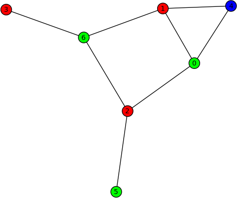
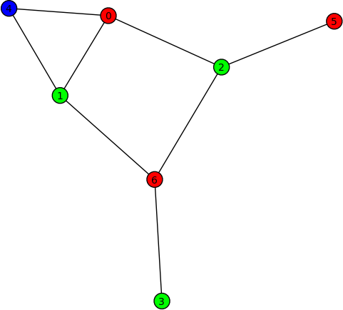
Graph colouring (Robert Miller) -- New method coloring() of the class sage.graphs.graph.Graph for obtaining the first (optimal) coloring found on a graph. Here are some examples on using this new method:
sage: G = Graph("Fooba")
sage: P = G.coloring()
sage: G.plot(partition=P)
sage: H = G.coloring(hex_colors=True)
sage: G.plot(vertex_colors=H)


- FIXME: summarize #6066
- FIXME: summarize #3932
- FIXME: summarize #5940
- FIXME: summarize #6086
Graphics
- FIXME: summarize #5249
- FIXME: summarize #4875
Group Theory
Improved efficiency of is_subgroup (Simon King) -- Testing whether a group is a subgroup of another group is now up to 2x faster than previously. The following timing statistics were obtained using the machine sage.math:
# BEFORE

sage: G = SymmetricGroup(7)
sage: H = SymmetricGroup(6)
sage: %time H.is_subgroup(G)
CPU times: user 4.12 s, sys: 0.53 s, total: 4.65 s
Wall time: 5.51 s
True
sage: %timeit H.is_subgroup(G)
10000 loops, best of 3: 118 µs per loop


# AFTER

sage: G = SymmetricGroup(7)
sage: H = SymmetricGroup(6)
sage: %time H.is_subgroup(G)
CPU times: user 0.00 s, sys: 0.00 s, total: 0.00 s
Wall time: 0.00 s
True
sage: %timeit H.is_subgroup(G)
10000 loops, best of 3: 56.3 µs per loop
Interfaces
Viewing Sage objects with a PDF viewer (Nicolas Thiery) -- Implements the option viewer="pdf" for the command view() so that one can invoke this command in the form view(object, viewer="pdf") in order to view object using a PDF viewer. Typical uses of this new optional argument include:
- You prefer to use a PDF viewer rather than a DVI viewer.
- You want to view LaTeX snippets which are not displayed well in DVI viewers (e.g. graphics produced using tikzpicture).
Change name of Pari's sum function when imported (Craig Citro) -- When Pari's sum function is imported, it is renamed to pari_sum in order to avoid conflict Python's sum function.
Linear Algebra
Improved performance for the generic linear_combination_of_rows and linear_combination_of_columns functions for matrices (William Stein) -- The speed-up for the generic functions linear_combination_of_rows and linear_combination_of_columns is up to 4x. The following timing statistics were obtained using the machine sage.math:
# BEFORE

sage: A = random_matrix(QQ, 50)
sage: v = [1..50]
sage: %timeit A.linear_combination_of_rows(v);
1000 loops, best of 3: 1.99 ms per loop
sage: %timeit A.linear_combination_of_columns(v);
1000 loops, best of 3: 1.97 ms per loop


# AFTER

sage: A = random_matrix(QQ, 50)
sage: v = [1..50]
sage: %timeit A.linear_combination_of_rows(v);
1000 loops, best of 3: 436 µs per loop
sage: %timeit A.linear_combination_of_columns(v);
1000 loops, best of 3: 457 µs per loop
Massively improved performance for 4 x 4 determinants (Tom Boothby) -- The efficiency of computing the determinants of 4 x 4 matrices can range from 16x up to 58,083x faster than previously, depending on the base ring. The following timing statistics were obtained using the machine sage.math:
# BEFORE

sage: S = MatrixSpace(ZZ, 4)
sage: M = S.random_element(1, 10^8)
sage: timeit("M.det(); M._clear_cache()")
625 loops, best of 3: 53 µs per loop
sage: M = S.random_element(1, 10^10)
sage: timeit("M.det(); M._clear_cache()")
625 loops, best of 3: 54.1 µs per loop
sage:
sage: M = S.random_element(1, 10^200)
sage: timeit("M.det(); M._clear_cache()")
5 loops, best of 3: 121 ms per loop
sage: M = S.random_element(1, 10^300)
sage: timeit("M.det(); M._clear_cache()")
5 loops, best of 3: 338 ms per loop
sage: M = S.random_element(1, 10^1000)
sage: timeit("M.det(); M._clear_cache()")
5 loops, best of 3: 9.7 s per loop


# AFTER

sage: S = MatrixSpace(ZZ, 4)
sage: M = S.random_element(1, 10^8)
sage: timeit("M.det(); M._clear_cache()")
625 loops, best of 3: 3.17 µs per loop
sage: M = S.random_element(1, 10^10)
sage: timeit("M.det(); M._clear_cache()")
625 loops, best of 3: 3.44 µs per loop
sage:
sage: M = S.random_element(1, 10^200)
sage: timeit("M.det(); M._clear_cache()")
625 loops, best of 3: 15.3 µs per loop
sage: M = S.random_element(1, 10^300)
sage: timeit("M.det(); M._clear_cache()")
625 loops, best of 3: 27 µs per loop
sage: M = S.random_element(1, 10^1000)
sage: timeit("M.det(); M._clear_cache()")
625 loops, best of 3: 167 µs per loop
Refactor matrix kernels (Rob Beezer) -- The core section of kernel computation for each (specialized) class is now moved into the method right_kernel(). Mostly these would replace kernel() methods that are computing left kernels. A call to kernel() or left_kernel() should arrive at the top of the hierarchy where it would take a transpose and call the (specialized) right_kernel(). So there wouldn't be a change in behavior in routines currently calling kernel() or left_kernel(), and Sage's preference for the left is retained by having the vanilla kernel() give back a left kernel. The speed-up for the computation of left kernels is up to 5% faster, and the computation of right kernels is up to 31% by eliminating paired transposes. The followingn timing statistics were obtained using sage.math:
# BEFORE

sage: n = 2000
sage: entries = [[1/(i+j+1) for i in srange(n)] for j in srange(n)]
sage: mat = matrix(QQ, entries)
sage: %time mat.left_kernel();
CPU times: user 21.92 s, sys: 3.22 s, total: 25.14 s
Wall time: 25.26 s
sage: %time mat.right_kernel();
CPU times: user 23.62 s, sys: 3.32 s, total: 26.94 s
Wall time: 26.94 s


# AFTER

sage: n = 2000
sage: entries = [[1/(i+j+1) for i in srange(n)] for j in srange(n)]
sage: mat = matrix(QQ, entries)
sage: %time mat.left_kernel();
CPU times: user 20.87 s, sys: 2.94 s, total: 23.81 s
Wall time: 23.89 s
sage: %time mat.right_kernel();
CPU times: user 18.43 s, sys: 0.00 s, total: 18.43 s
Wall time: 18.43 s
- FIXME: summarize #5554
Miscellaneous
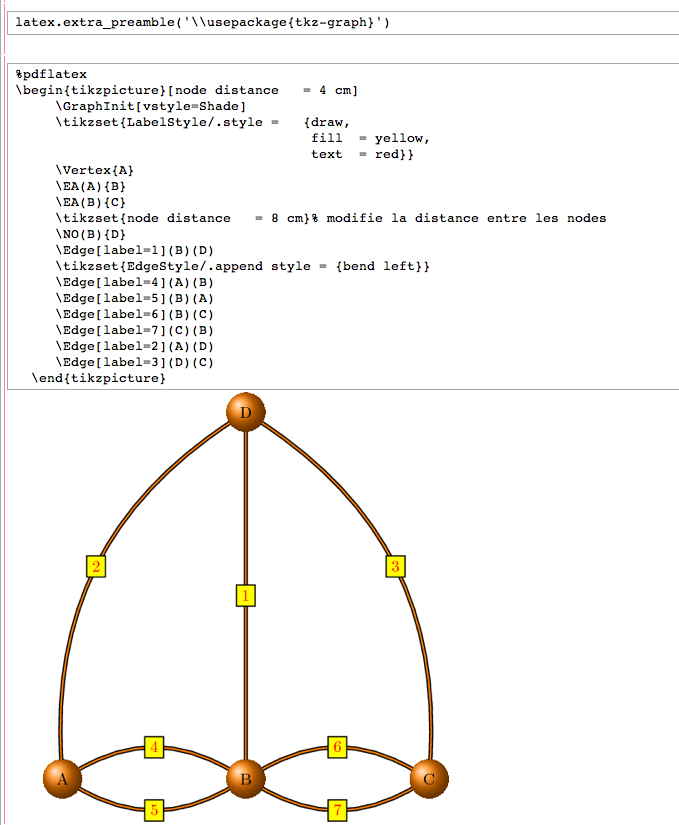
Allow use of pdflatex instead of latex (John Palmieri) -- One can now use pdflatex instead of latex in two different ways:
Use a %pdflatex cell in a notebook; or
Call latex.pdflatex(True)
after which any use of latex (in a %latex cell or using the view command) will use pdflatex. One visually appealing aspect of this is that if you have the most recent version of pgf installed, as well as the tkz-graph package, you can produce images like the following:

- FIXME: summarize #5783
- FIXME: summarize #5796
- FIXME: summarize #5120
Modular Forms
Action of Hecke operators on Gamma_1(N) modular forms (David Loeffler) -- Here's an example:
sage: ModularForms(Gamma1(11), 2).hecke_matrix(2)

[       -2         0         0         0         0         0         0         0         0         0]
[        0      -381         0      -360         0       120     -4680     -6528     -1584      7752]
[        0      -190         0      -180         0        60     -2333     -3262      -789      3887]
[        0   -634/11         1   -576/11         0    170/11  -7642/11 -10766/11      -231  12555/11]
[        0     98/11         0     78/11         0    -26/11   1157/11   1707/11        30  -1959/11]
[        0    290/11         0    271/11         0    -50/11   3490/11   5019/11        99  -5694/11]
[        0    230/11         0    210/11         0    -70/11   2807/11   3940/11        84  -4632/11]
[        0    122/11         0    120/11         1    -40/11   1505/11   2088/11        48  -2463/11]
[        0     42/11         0     46/11         0    -30/11    554/11    708/11        21   -970/11]
[        0     10/11         0     12/11         0      7/11    123/11    145/11         7   -177/11]
- FIXME: summarize #6019
- FIXME: summarize #5924
Notebook
Number Theory
- FIXME: summarize #5250
- FIXME: summarize #6013
- FIXME: summarize #6008
- FIXME: summarize #6004
- FIXME: summarize #6059
- FIXME: summarize #6064
Numerical
Packages
- FIXME: summarize #4223
- FIXME: summarize #6031
- FIXME: summarize #5934
- FIXME: summarize #1338
- FIXME: summarize #6032
- FIXME: summarize #6024
P-adics
- FIXME: summarize #5105
- FIXME: summarize #5236
Quadratic Forms
- FIXME: summarize #6037
Symbolics
- FIXME: summarize #5777
- FIXME: summarize #5930
Topology
Random simplicial complexes (John Palmieri) -- New method RandomComplex() in the module sage/homology/examples.py for producing a random d-dimensional simplicial complex on n vertices. Here's an example:
sage: simplicial_complexes.RandomComplex(6,12)
Simplicial complex with vertex set (0, 1, 2, 3, 4, 5, 6, 7) and facets {(0, 1, 2, 3, 4, 5, 6, 7)}
User Interface
